First we will describe Gradient Descent in \(\wR^3\). Once we understand the geometry, it is easy to generalize to \(\mathbb{R}^n\). Once we understand general Gradient Descent, Stochastic Gradient Descent will follow quickly.
For general Gradient Descent, we want to find the direction of steepest descent. That is, suppose we are standing on the side of a mountain and that we wish to go down the mountain side in the shortest possible path. Also suppose that we are blindfolded (we probably shouldn’t be mountain climbing blindfolded but anyway). How can we determine which direction to go in?
We will need to develop a few tools to do this: tangent plane, approximation formula, and directional derivative.
Tangent Plane
Recall that there are a few ways to represent a plane in \(\mathbb{R}^3\):
$$ A(x - x_0) + B(y - y_0) + C(w - w_0) = 0 $$
$$ A x + B y + C w = D $$
$$ w = D + A x + B y $$
It is easy to convert between each representation and each representation can be useful for different situations. Here we will use the first form. This is called the point-normal form.
Suppose we have a function \(w=f(x,y)\) of two variables. How can we select the plane that is tangent to \(w=f(x,y)\) at the point \((x_0, y_0)\)? The tangent must
(1) pass through the point \(P=(x_0, y_0, w_0)\) where \(w_0=f(x_0, y_0)\).
(2) contain the tangent lines to the graphs of the two partial functions. This will hold if the plane has the same slopes in the \(\mathbf{i}\) and \(\mathbf{j}\) directions as the surface of \(w=f(x,y)\).
This is easy to understand when we look at a picture:
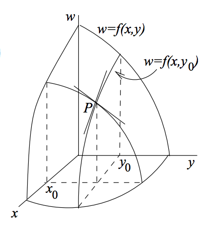
We can see the tangent lines to the graphs of the two partial functions. They form a cross at the point \(P=(x_0, y_0, w_0)\). One of these tangent lines has the same slope as that of the surface in the direction of \(\mathbf{i}\). And the other tangent line has the same slope as that of the surface in the direction of \(\mathbf{j}\). The tangent plane that we want will simply be the linear combinations of those two tangent lines.
Using conditions (1) and (2), we can easily derive the equation for the tangent plane. The general equation of the plane through \(P=(x_0, y_0, w_0)\) is
$$ A(x - x_0) + B(y - y_0) + C(w - w_0) = 0 $$
But how can we determine what \(A\), \(B\), and \(C\) are? Assume the plane is not vertical. Then \(C\neq0\) and we can divide through by it
$$ \frac{A}{C}(x - x_0) + \frac{B}{C}(y - y_0) + (w - w_0) = 0 $$
Let \(a=\frac{A}{C}\) and \(b=\frac{B}{C}\) and rewrite this as
$$ w - w_0=a(x - x_0) + b(y - y_0) $$
This plane passes through \(P=(x_0, y_0, w_0)\). What values of \(a\) and \(b\) will make it tangent to the graph of \(w=f(x,y)\) at the point \(P=(x_0, y_0, w_0)\)? Well \(a\) must be the slope of the graph in the \(\mathbf{i}\) direction at the point \(P=(x_0, y_0, w_0)\). And \(b\) must be the slope of the graph in the \(\mathbf{j}\) direction at the point \(P=(x_0, y_0, w_0)\).
But these are just the slopes of the tangent lines to the two partial functions. And of course these slopes are just the partial functions evaluated at \((x_0, y_0)\). Let’s write this clearly:
$$ \frac{\partial f}{\partial x}\bigbar_{(x_0,y_0)}= \begin{cases} \text{the slope of the graph of }f(x,y)\text{ at the point }(x_0, y_0)\text{ in the }\mathbf{i}\text{ direction}\\ \text{the slope of the tangent line to the partial function }\frac{\partial f}{\partial x}\text{ at the point }(x_0, y_0)\end{cases} $$
$$ \frac{\partial f}{\partial y}\bigbar_{(x_0,y_0)}= \begin{cases} \text{the slope of the graph of }f(x,y)\text{ at the point }(x_0, y_0)\text{ in the }\mathbf{j}\text{ direction}\\ \text{the slope of the tangent line to the partial function }\frac{\partial f}{\partial y}\text{ at the point }(x_0, y_0)\end{cases} $$
Hence we set \(a=\frac{\partial f}{\partial x}(x_0,y_0)\) and \(b=\frac{\partial f}{\partial y}(x_0,y_0)\) and condition (2) is now satisfied. That is, this plane
$$ w - w_0=\frac{\partial f}{\partial x}\Big|_{(x_0,y_0)}(x - x_0) + \frac{\partial f}{\partial y}\Big|_{(x_0,y_0)}(y - y_0) $$
is the tangent plane to \(w=f(x,y)\) at the point \(P=(x_0, y_0, w_0)\).
Approximation Formula
What’s really cool about the tangent plane is that it gives us a good approximation to the function \(f(x,y)\) for all points \((x,y)\) near the point \((x_0, y_0)\). That is,
$$ \begin{equation} \forall(x,y)\approx(x_0,y_0):\quad f(x,y)\approx w_0+\frac{\partial f}{\partial x}\Big|_{(x_0,y_0)}(x - x_0) + \frac{\partial f}{\partial y}\Big|_{(x_0,y_0)}(y - y_0) \tag{1}\end{equation} $$
This is often called the linearization of \(f(x,y)\) at \((x_0,y_0)\); it is the linear function which gives the best approximation to \(f(x,y)\) for all \((x,y)\) near \((x_0,y_0)\). Notice that the right hand side of (1) is just the equation of the tangent plane. Of course this is just the first-order Taylor approximation.
Using \(\Delta\) notation, we can put
$$ \Delta x\equiv x-x_0 \quad \Delta y\equiv y-y_0 \quad \Delta w\equiv w-w_0 $$
and write (1) as
$$ \begin{equation} \Delta w\approx\frac{\partial f}{\partial x}\Big|_{(x_0,y_0)}\Delta x+\frac{\partial f}{\partial y}\Big|_{(x_0,y_0)}\Delta y \quad \forall(x,y)\approx(x_0,y_0) \tag{2}\end{equation} $$
With some abuse of notation, this can be written as
$$ \begin{equation} \Delta f\approx\frac{\partial f}{\partial x}\Delta x+\frac{\partial f}{\partial y}\Delta y \tag{3}\end{equation} $$
where it is understood that the partial derivatives are evaluated at some point \((x_0,y_0)\) and that this holds for all \((x,y)\) sufficiently close to \((x_0,y_0)\).
This can be written even more compactly. Define
$$ \begin{equation} \nabla f\equiv\begin{bmatrix} \frac{\partial f}{\partial x}\\\frac{\partial f}{\partial y} \end{bmatrix} \quad \Delta \mathbf{v}\equiv\begin{bmatrix} \Delta x\\\Delta y \end{bmatrix} \end{equation} $$
Of course \(\nabla f\) is the typical gradient. Now (3) can be written as
$$ \begin{equation} \Delta f\approx\nabla f\cdot\Delta\mathbf{v} \tag{4}\end{equation} $$
where, again, it is understood that the partial derivatives are evaluated at some point \((x_0,y_0)\) and that this holds for sufficiently small \(\Delta\mathbf{v}\).
Suppose instead that \(f(\mathbf{v})\) is a function of \(n\) variables. Then define
$$ \nabla f\equiv\begin{bmatrix} \frac{\partial f}{\partial v_1}\\\vdots\\\frac{\partial f}{\partial v_n} \end{bmatrix} \quad \mathbf{v}\equiv\begin{bmatrix} v_1\\\vdots\\v_n \end{bmatrix} \quad \mathbf{v_0}\equiv\begin{bmatrix} v_{0,1}\\\vdots\\v_{0,n} \end{bmatrix} \quad \Delta \mathbf{v}\equiv\begin{bmatrix} v_1-v_{0,1}\\\vdots\\v_n-v_{0,n} \end{bmatrix}\equiv\begin{bmatrix} \Delta v_1\\\vdots\\\Delta v_n \end{bmatrix} =\mathbf{v}-\mathbf{v_0} $$
so that (4) remains the same
$$ \Delta f\approx\nabla f\cdot\Delta\mathbf{v} $$
Directional Derivative
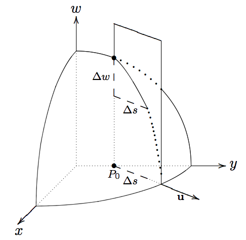
OK, one last tool and then we dig into Gradient Descent. We define the directional derivative of \(w=f(x,y)\) at a point \(P_0=(x_0,y_0)\) in the xy-plane (in \(\mathbb{R}^3\)) in the direction \(\mathbf{u}\) as
$$ \frac{df}{ds}\Big|_{P_0,\mathbf{u}}\equiv \lim_{\Delta s\rightarrow0}\frac{\Delta f}{\Delta s} $$
\(\Delta f=\Delta w\) is the change in \(f\) caused by a step (starting at \(P_0\)) of length \(\Delta s\) in the direction of \(\mathbf{u}\) (in the xy-plane). This picture should make clear the definition that we just stated. We can see that \(\Delta s\) is just a (short) line segment starting at \(P_0\) and in the direction of \(\mathbf{u}\).
So the directional derivative is just like the typical derivative of a function of one variable except that we define it for a specific direction. Rather than using a limit, there is a more convenient way to express this:
$$ \begin{equation} \frac{df}{ds}\Big|_{P_0,\mathbf{u}}\equiv \lim_{\Delta s\rightarrow0}\frac{\Delta f}{\Delta s}= \nabla f\Big|_{P_0}\cdot\mathbf{u} \tag{5}\end{equation} $$
Let’s prove (5). It will come in very handy. To prove (5), a picture will be helpful:
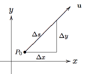
This picture shows the change in position from \(P_0\) to another point after taking a step of length \(\Delta s\) in the direction of \(\mathbf{u}\). We can see that the edges \(\Delta s\), \(\Delta x\), and \(\Delta y\) form a right triangle. So the Pythagorean Theorem tells us that
$$ (\Delta s)^2=(\Delta x)^2+(\Delta y)^2 $$
We can divide through by \((\Delta s)^2\) so that
$$ 1=\frac{(\Delta x)^2}{(\Delta s)^2}+\frac{(\Delta y)^2}{(\Delta s)^2} =\Big(\frac{\Delta x}{\Delta s}\Big)^2+\Big(\frac{\Delta y}{\Delta s}\Big)^2 $$
Set \(\mathbf{u}=\begin{bmatrix} \frac{\Delta x}{\Delta s}&\frac{\Delta y}{\Delta s} \end{bmatrix}^T\) so that \(\mathbf{u}\) is a unit vector:
$$ \norm{\mathbf{u}}= \sqrt{\mathbf{u}^T\mathbf{u}}= \sqrt{\Big(\frac{\Delta x}{\Delta s}\Big)^2+\Big(\frac{\Delta y}{\Delta s}\Big)^2} =1 $$
The tangent plane approximation to \(f\) at \(P_0\) is
$$ \Delta f\approx \frac{\partial f}{\partial x}\Big|_{P_0}\Delta x+\frac{\partial f}{\partial y}\Big|_{P_0}\Delta y $$
Dividing this approximation by \(\Delta s\) gives
$$ \frac{\Delta f}{\Delta s}\approx \frac{\partial f}{\partial x}\Big|_{P_0}\frac{\Delta x}{\Delta s}+ \frac{\partial f}{\partial y}\Big|_{P_0}\frac{\Delta y}{\Delta s} $$
Just as we did earlier, we can write the right hand side as a dot product:
$$ \frac{\Delta f}{\Delta s}\approx\nabla f\Big|_{P_0}\cdot\mathbf{u} $$
Finally, we let \(\Delta s\) go to \(0\) and we get
$$ \begin{equation} \frac{df}{ds}\Big|_{P_0,\mathbf{u}}= \nabla f\Big|_{P_0}\cdot\mathbf{u} \end{equation} $$
which is what we wanted to prove.
Gradient Descent
OK, back to our original problem. We’re blindfolded on a mountain side. We want to go down the mountain as quickly as possible. Which direction should we go? Well, we could take a step in every direction and see which step goes down the most. But that would take a long time. Instead, we can use directional derivatives to tell us the steepest step downwards!
We will prove that the direction of steepest descent is \(-\nabla f\). After all the math we just did, you might suspect this will be a long, complicated proof. In fact, all the work we just did will allow us to prove this in a few lines.
Let \(\mathbf{v}\) be some undetermined unit vector in \(\mathbb{R}^n\) and let \(f\) be a real valued, differentiable function defined on \(\mathbb{R}^n\). We already know that the derivative of \(f\) in the direction of \(\mathbf{v}\) is \(~\frac{df}{ds}\bigbar_\mathbf{v}=\nabla f\cdot\mathbf{v}\). Let \(\theta\) be the angle between \(\nabla f\) and \(\mathbf{v}\). There is a formula that relates the \(\cos(\theta)\) with the dot product of \(\nabla f\) and \(\mathbf{v}\):
$$ \nabla f\cdot\mathbf{v}=\norm{\nabla f}\norm{\mathbf{v}}\cos(\theta) =\norm{\nabla f}\cos(\theta) $$
The last equality follows from \(\norm{\mathbf{v}}=1\). So the question is, which \(\mathbf{v}\) will minimize \(\nabla f\cdot\mathbf{v}=\norm{\nabla f}\cos(\theta)\)? Since \(\theta\) is the angle between \(\nabla f\) and \(\mathbf{v}\), we can select \(\mathbf{v}\) to minimize \(\cos(\theta)\) and we’ll be done. Well, the cosine function has a minimum value of -1 when \(\theta=\pi\). That is, the direction of steepest descent is \(180^\circ\) from the direction of \(\nabla f\). But that’s just \(-\nabla f\).
Stochastic Gradient Descent
This section might seem anticlimactic. We’ve already done the heavy lifting. We know how to do Gradient Descent. We know which direction will take us “down” a function as fast as possible. But we really only solved this for one small increment. General Gradient Descent only tells you which small, next step is the steepest. It doesn’t tell you how to get all the way down the mountain or even how to get to a valley in the mountains. We need a way to find local maxima and minima or possibly global maxima and minima.
Let’s summarize the situation. We collect some data, we select a loss function, and we select the hyperparameters including the learning rate \(\eta\). Here’s what we do at each iteration:
- Forward propogate
- Compute the loss
- Backpropogate to get the gradients of the weights and biases
- Update the weights and biases: for each weight matrix and bias matrix P, perform $$P~-=\eta\cdot\nabla P$$
We know \(-\nabla P\) will provide the steepest descent for a small step for the chosen loss function. The learning rate \(\eta\) allows us to calibrate the length of our steps. And that’s really it.