Backpropagation
Backpropagation is the application of the multivariable chain rule (from Calculus) to the computation graph of a neural network. This series of videos is a good review of the multivariable chain rule.
The form of the multivariable chain rule that we need is as follows. Suppose $f:\wR^2\mapsto\wR$ is differentiable and suppose $v:\wR\mapsto\wR^2$ is differentiable. Then the composition $(f\circ v):\wR\mapsto\wR$ is differentiable and
$$ \wpart{(f\circ v)}{t}=\wpart{f}{v_1}\wpart{v_1}{t}+\wpart{f}{v_2}\wpart{v_2}{t} $$
We have denoted the composition of two functions with the symbol $\circ$. We will also use this symbol to denote the Hadamard product. The context makes the meaning unambiguous.
Suppose we have training data $\set{x^{(i)},y^{(i)}}_{i=1}^{m}$ and suppose we build a fully-connected neural network with $L+1$ layers, numbered as $0,1,\dots,L$. Let $n_l$ denote the number of neurons in layer $l$. For $l=1,\dots,L$, let $W^l$ denote the weight matrix from layer $l-1$ to layer $l$ and let $b^l$ denote the bias vector from layer $l-1$ to layer $l$. Then
$$ W^l\equiv\pmtrx{w_{1,1}^{l}&\dotsb&\dotsb&w_{1,n_{l-1}}^l\\\vdots&\ddots&\ddots&\vdots\\w_{n_{l},1}^l&\dotsb&\dotsb&w_{n_{l},n_{l-1}}^l} \dq\dq b^l\equiv\pmtrx{b_1^l\\\vdots\\b_{n_l}^{l}} $$
For $l=1,\dots,L$, let $z_j^l$ denote the weighted input to the $j^{th}$ neuron in layer $l$ and let $g^l:\wR\mapsto\wR$ denote the activation for the $l^{th}$ layer.
For $l=0,\dots,L$, let $a_j^l$ denote the output of the $j^{th}$ neuron in layer $l$. Then $a_j^0=x_j$ or $a^0=x$. And, for $l=1,\dots,L$, we have $a_j^l=g^l(z_j^l)$ or $a^l=g^l(z^l)$. Hence
$$ z_j^l=\sum_{k=1}^{n_{l-1}}w_{j,k}^la_k^{l-1}+b_j^l \dq\iff\dq z^l=W^la^{l-1}+b^l $$
In more detail, we have
$$\align{ z^l &= W^la^{l-1}+b^l \\ &= \pmtrx{w_{1,1}^l&\dotsb&\dotsb&w_{1,n_{l-1}}^l\\\vdots&\ddots&\ddots&\vdots\\w_{n_l,1}^l&\dotsb&\dotsb&w_{n_l,n_{l-1}}^l} \pmtrx{a_1^{l-1}\\\vdots\\\vdots\\a_{n_{l-1}}^{l-1}}+\pmtrx{b_1^l\\\vdots\\b_{n_l}^{l}} \\ &= \pmtrx{\sum_{k=1}^{n_{l-1}}w_{1,k}^la_k^{l-1}\\\vdots\\\sum_{k=1}^{n_{l-1}}w_{n_l,k}^la_k^{l-1}}+\pmtrx{b_1^l\\\vdots\\b_{n_l}^{l}} \\ &= \pmtrx{\sum_{k=1}^{n_{l-1}}w_{1,k}^la_k^{l-1}+b_1^l\\\vdots\\\sum_{k=1}^{n_{l-1}}w_{n_l,k}^la_k^{l-1}+b_{n_l}^l} \\ }$$
For instance, if $L=3$, $n_0=3$, $n_1=5$, $n_2=4$, and $n_3=2$, then our computation graph is
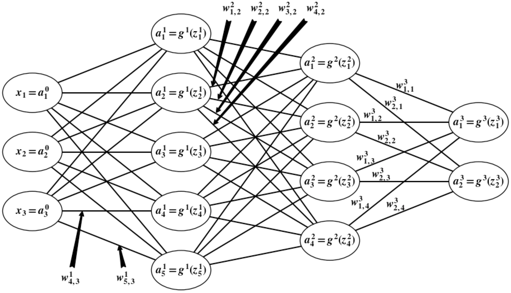
In this case, we have
$$ W^3\equiv\pmtrx{w_{1,1}^{3}&w_{1,2}^3&w_{1,3}^3&w_{1,4}^3\\w_{2,1}^{3}&w_{2,2}^3&w_{2,3}^3&w_{2,4}^3} $$
Note that the $1^{st}$ row of $W^3$ maps the outputs of all neurons in layer $2$ to the weighted input of the $1^{st}$ neuron in layer $3$. Also note that the $1^{st}$ column of $W^3$ maps the output of the $1^{st}$ neuron of layer $2$ to the weighted inputs of each neuron in layer $3$.
Let $\lossfnsm$ denote our loss function. We need to make a couple of assumptions about $\lossfnsm$. The first assumption we need is that $\lossfnsm$ can be written as a linear combination of the loss functions $\lossfnsm_i$ for each observation $x^{(i)},y^{(i)}$ in the training data. That is, let $\theta$ denote the list of all weight matrices and bias vectors:
$$ \theta\equiv W^1,\dots,W^{L},b^1,\dots,b^{L} $$
Then our assumption is that there exist scalars $c_1,\dots,c_m$ such that, for all values of $\theta$, we have
$$ \lossfn{\theta}=\sum_{i=1}^mc_i\lossfnsm_i(\theta) $$
Note that the scalars $c_1,\dots,c_m$ are fixed for a valid loss function and do not depend on $\theta$.
Now recall that the differentiation map $\partial/\partial W^l$ is linear. Hence, if we can compute $\partial\lossfnsm_i/\partial W^l$ for each observation $i$ and each layer $l$, then we can compute
$$ \wpart{\lossfn{\theta}}{W^l}=\wpart{}{W^l}\prnfit{\sum_{i=1}^mc_i\lossfnsm_i(\theta)}=\sum_{i=1}^mc_i\wpart{\lossfnsm_i(\theta)}{W^l} $$
for each layer $l$. Hence, our goal is to find convenient formulas for $\partial\lossfnsm_i/\partial W^l$ and $\partial\lossfnsm_i/\partial b^l$. Going forward, for cleaner notation, we will drop the subscript $i$ from $\lossfnsm_i$ but we’ll keep in mind that we’re actually working with the loss function of a single observation - unless the context makes it clear that the loss function is with respect to all observations.
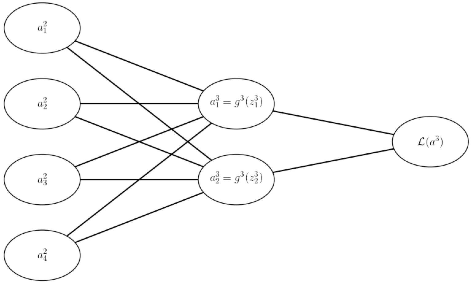
The second assumption we need to make is that the loss function (of a single observation) can be written as a function of the outputs $a^L$ from the neural network. Using our example from above, we extend the computation graph:
Now we’re ready for the backpropagation algorithm:
Proposition Backpropagation Define
$$ \delta_j^{l}\equiv\wpart{\lossfnsm}{z_j^{l}} \dq\iff\dq \delta^l\equiv\nabla_{z^l}\lossfnsm \tag{BP.0} $$
Then
$$ \delta^{L}=\nabla_{a_L}\lossfnsm\hdmrdprd(g^L)'(z^L) \tag{BP.A} $$
$$ \delta^{l}=\prn{(W^{l+1})^T\delta^{l+1}}\hdmrdprd(g^l)'(z^l) \tag{BP.B} $$
$$ \nabla_{a^l}\lossfnsm = (W^{l+1})^T\delta^{l+1} \tag{BP.C} $$
$$ \nabla_x\lossfnsm=(W^{1})^T\delta^{1} \tag{BP.D} $$
$$ \wpart{\lossfnsm}{W^l}=\delta^l(a^{l-1})^T \tag{BP.E} $$
$$ \nabla_{b^l}\lossfnsm = \delta^l \tag{BP.F} $$
Proof First note that we are slightly abusing notation by writing $\partial\lossfnsm/\partial z_j^L$ since $\lossfnsm$ is a function of the output activations $a_1^L,\dots,a_{n_L}^L$ and not directly a function of $z_j^L$. Since $\lossfnsm(a^L)=\lossfnsm\prn{a^L(z^L)}=(\lossfnsm\circ a^L)(z^L)$, then
$$ \delta_j^{L}=\wpart{\lossfnsm}{z_j^L}=\wpart{(\lossfnsm\circ a^L)}{z_j^L}=\sum_{k=1}^{n_L}\wpart{\lossfnsm}{a_k^L}\wpart{a_k^L}{z_j^L}=\wpart{\lossfnsm}{a_j^L}\wpart{a_j^L}{z_j^L}=\wpart{\lossfnsm}{a_j^L}(g^L)'(z_j^L) $$
The fourth equality follows because $a_k^L=g^L(z_k)$ depends on $z_j^L$ if and only if $k=j$. Hence $\partial a_k^L\big/\partial z_j^L=0$ for $k\neq j$. Said another way, there is exactly one path from $\lossfnsm(a^L)$ to $z_j^L$. This is easy to see in the computation graphs above. Hence
$$ \delta^L=\pmtrx{\delta_1^{L}\\\vdots\\\delta_{n_L}^{L}}=\pmtrx{\wpart{\lossfnsm}{a_1^L}(g^L)'(z_1^L)\\\vdots\\\wpart{\lossfnsm}{a_{n_L}^L}(g^L)'(z_{n_L}^L)} =\pmtrx{\wpart{\lossfnsm}{a_1^L}\\\vdots\\\wpart{\lossfnsm}{a_{n_L}^L}}\hdmrdprd\pmtrx{(g^L)'(z_1^L)\\\vdots\\(g^L)'(z_{n_L}^L)} =\nabla_{a_L}\lossfnsm\hdmrdprd(g^L)'(z^L) $$
Next, for all $i=1,\dots,n_{l+1}$, note that
$$ z_i^{l+1}=\sum_{k=1}^{n_l}w_{i,k}^{l+1}a_k^l+b_i^{l+1}=\sum_{k=1}^{n_l}w_{i,k}^{l+1}g^l(z_k^l)+b_i^{l+1} $$
Now fix $j$ and consider the weighted input $z_j^l$ for the $j^{th}$ neuron in the $l^{th}$ layer. The second equality shows that, for all $i=1,\dots,n_{l+1}$, the value $z_i^{l+1}$ depends on $z_j^l$. That is, the input for every neuron in layer $l+1$ depends on the input for every neuron in layer $l$. This is to be expected from a fully-connected network. Hence
$$ \delta_j^l=\wpart{\lossfnsm}{z_j^l}=\sum_{i=1}^{n_{l+1}}\wpart{\lossfnsm}{z_i^{l+1}}\wpart{z_i^{l+1}}{z_j^l}=\sum_{i=1}^{n_{l+1}}\delta_i^{l+1}w_{i,j}^{l+1}(g^l)'(z_j^l)=(g^l)'(z_j^l)\sum_{i=1}^{n_{l+1}}w_{i,j}^{l+1}\delta_i^{l+1} $$
where the fourth equality follows from $\delta_i^{l+1}=\partial\lossfnsm/\partial z_i^{l+1}$ and
$$ \wpart{z_i^{l+1}}{z_j^l}=\wpart{}{z_j^l}\prnfit{\sum_{k=1}^{n_l}w_{i,k}^{l+1}g^l(z_k^l)+b_i^{l+1}}=\sum_{k=1}^{n_l}\wpart{}{z_j^l}\prnfit{w_{i,k}^{l+1}g^l(z_k^l)+b_i^{l+1}}=w_{i,j}^{l+1}(g^l)'(z_j^l) $$
Hence
$$\align{ \delta^{l} &= \pmtrx{\delta_1^l\\\vdots\\\vdots\\\delta_{n_l}^l} \\ &= \pmtrx{(g^l)'(z_1^l)\sum_{i=1}^{n_{l+1}}w_{i,1}^{l+1}\delta_i^{l+1}\\\vdots\\\vdots\\(g^l)'(z_{n_l}^l)\sum_{i=1}^{n_{l+1}}w_{i,{n_l}}^{l+1}\delta_i^{l+1}} \\ &= \pmtrx{\sum_{i=1}^{n_{l+1}}w_{i,1}^{l+1}\delta_i^{l+1}\\\vdots\\\vdots\\\sum_{i=1}^{n_{l+1}}w_{i,{n_l}}^{l+1}\delta_i^{l+1}} \hdmrdprd\pmtrx{(g^l)'(z_1^l)\\\vdots\\\vdots\\(g^l)'(z_{n_l}^l)} \\ &= \cbrfit{\pmtrx{w_{1,1}^{l+1}&\dotsb&w_{n_{l+1},1}^{l+1}\\\vdots&\ddots&\vdots\\\vdots&\ddots&\vdots\\w_{1,n_l}^{l+1}&\dotsb&w_{n_{l+1},n_l}^{l+1}}\pmtrx{\delta_1^{l+1}\\\vdots\\\delta_{n_{l+1}}^{l+1}}}\hdmrdprd(g^l)'\pmtrx{z_1^l\\\vdots\\\vdots\\z_{n_l}^l} \\ &= \prn{(W^{l+1})^T\delta^{l+1}}\hdmrdprd(g^l)'(z^l) }$$
Similarly
$$ \wpart{z_i^{l+1}}{a_j^l}=\wpart{}{a_j^l}\prnfit{\sum_{k=1}^{n_l}w_{i,k}^{l+1}a_k^l+b_i^{l+1}}=w_{i,j}^{l+1} $$
Hence
$$ \wpart{\lossfnsm}{a_j^l}=\sum_{i=1}^{n_{l+1}}\wpart{\lossfnsm}{z_i^{l+1}}\wpart{z_i^{l+1}}{a_j^l}=\sum_{i=1}^{n_{l+1}}\delta_i^{l+1}w_{i,j}^{l+1} $$
Hence
$$ \nabla_{a^l}\lossfnsm = \pmtrx{\wpart{\lossfnsm}{a_1^l}\\\vdots\\\vdots\\\wpart{\lossfnsm}{a_{n_l}^l}} = \pmtrx{\sum_{i=1}^{n_{l+1}}w_{i,1}^{l+1}\delta_i^{l+1}\\\vdots\\\vdots\\\sum_{i=1}^{n_{l+1}}w_{i,{n_l}}^{l+1}\delta_i^{l+1}} = \pmtrx{w_{1,1}^{l+1}&\dotsb&w_{n_{l+1},1}^{l+1}\\\vdots&\ddots&\vdots\\\vdots&\ddots&\vdots\\w_{1,n_l}^{l+1}&\dotsb&w_{n_{l+1},n_l}^{l+1}}\pmtrx{\delta_1^{l+1}\\\vdots\\\delta_{n_{l+1}}^{l+1}} = (W^{l+1})^T\delta^{l+1} $$
In particular
$$ \nabla_x\lossfnsm=\nabla_{a^0}\lossfnsm=(W^{0+1})^T\delta^{0+1}=(W^{1})^T\delta^{1} $$
Next, note that there are many paths in the computation graph from $\lossfn{a^L}$ to $W_{j,k}^l$. However, there is a single path from $z_j^l$ to $W_{j,k}^l$. Hence $\lossfnsm\prnfit{z_j^l(W_{j,k}^l)}=(\lossfnsm\circ z_j^l)(W_{j,k}^l)$ describes $\lossfnsm$ as a function of $W_{j,k}^l$ and the single variable chain rule gives
$$ \wpart{\lossfnsm}{W_{j,k}^l}=\wpart{\lossfnsm}{z_j^l}\wpart{z_j^l}{W_{j,k}^l}=\delta_j^l\wpart{}{W_{j,k}^l}\prnfit{\sum_{k=1}^{n_{l-1}}w_{j,k}^la_k^{l-1}+b_j^l}=\delta_j^l\sum_{k=1}^{n_{l-1}}\wpart{}{W_{j,k}^l}\prnfit{w_{j,k}^la_k^{l-1}+b_j^l}=\delta_j^la_k^{l-1} $$
Hence
$$\align{ \wpart{\lossfnsm}{W^l} &= \pmtrx{\wpart{\lossfnsm}{W_{1,1}^l}&\dotsb&\dotsb&\wpart{\lossfnsm}{W_{1,n_{l-1}}^l}\\\vdots&\ddots&\ddots&\vdots\\\wpart{\lossfnsm}{W_{n_l,1}^l}&\dotsb&\dotsb&\wpart{\lossfnsm}{W_{n_1,n_{l-1}}^l}} \\ &= \pmtrx{\delta_1^la_1^{l-1}&\dotsb&\dotsb&\delta_1^la_{n_{l-1}}^{l-1}\\\vdots&\ddots&\ddots&\vdots\\\delta_{n_l}^la_1^{l-1}&\dotsb&\dotsb&\delta_{n_l}^la_{n_{l-1}}^{l-1}} \\ &= \pmtrx{\delta_1^l\\\vdots\\\delta_{n_l}^l}\pmtrx{a_1^{l-1}&\dotsb&\dotsb&a_{n_{l-1}}^{l-1}} \\ &= \delta^l(a^{l-1})^T }$$
Similarly
$$ \wpart{\lossfnsm}{b_j^l}=\wpart{\lossfnsm}{z_j^l}\wpart{z_j^l}{b_j^l}=\delta_j^l $$
Hence
$$ \nabla_{b^l}\lossfnsm = \pmtrx{\wpart{\lossfnsm}{b_1^l}\\\vdots\\\wpart{\lossfnsm}{b_{n_l}^l}} = \pmtrx{\delta_1^l\\\vdots\\\delta_{n_l}^l} = \delta^l $$
$\wes$
Multilayer Perceptron
A Multilayer Perceptron (MLP) is a fully-connected neural network with at least three layers: the input layer, at least one hidden layer, and the output layer. By fully-connected, we mean that every neuron in layer $l$ is connected to every neuron in layer $l+1$ via a weight and bias.
Let’s construct a simple MLP. Suppose we have a data set where the target $y$ is binary, say $0$ or $1$. We will construct an MLP with an output layer that consists of a single neuron. We’ll use the sigmoid function, denoted $\sigma$, as the activation for the last layer since the sigmoid is a valid cumulative distribution function on $\wR$. Hence we interpret the output neuron for the $i^{th}$ observation to be correct if
$$ a_i^L=\sigma(z_i^L)\gt0.5\text{ and }y_i=1 \dq\text{or}\dq a_i^L=\sigma(z_i^L)\leq0.5\text{ and }y_i=0 \tag{MLP.0} $$
where $a_i^L$ and $z_i^L$ are the output and weighted input, respectively, to the single neuron in the output layer for the $i^{th}$ observation. Also, $y_i$ denotes the target value for the $i^{th}$ observation. Similarly, going forward, $x_i$ will denote the input neuron for the $i^{th}$ observation.
Let $\theta$ denote the collection of all weight matrices and bias vectors in the MLP. We know that $z_i^L$ is a function of $x_i$ parameterized by $\theta$. That is, we start with $x_i$ and apply the weights, biases, and activations in each successive layer to get $z_i^L$. Hence we can write $z_i^L=f_{\theta}(x_i)$ for some function $f_{\theta}$ that is parameterized by $\theta$. Hence we can define $h_{\theta}$ by
$$ h_{\theta}(x_i) \equiv \sigma(f_{\theta}(x_i)) = \sigma(z_i^L) $$
Then the probablistic interpretation of an MLP is
$$\align{ &P(y_i=1\mid x_i;\theta) = h_\theta(x_i) = \sigma(z_i^L)\\\\ &P(y_i=0\mid x_i;\theta) = 1-h_\theta(x_i) = 1 - \sigma(z_i^L)\\\\ }$$
This notation indicates that this is the distribution of $y_i$ given $x_i$ parameterized by $\theta$. That is, we are conditioning on $x_i$ but we’re parameterizing (not conditioning on) the fixed value $\theta$. This can be written more compactly:
$$ P(y_i\mid x_i;\theta) = \prn{\sigma(z_i^L)}^{y_i}\prn{1-\sigma(z_i^L)}^{1-y_i}\tag{MLP.1} $$
The goal of an MLP is this: Given $X=x_1,\dots,x_m$ (the design matrix), what is the probability distribution of $y=y_1,\dots,y_m$? The probability is denoted by $P(y\mid X;\theta)$. This quantity is typically viewed as a function of $y$ (and perhaps $X$), for a fixed value of $\theta$. When we wish to explicitly view this as a function of $\theta$, we will instead call it the likelihood function:
$$ L(\theta)=L(\theta;X,y) = P(y\mid X;\theta) $$
The key assumption of the probablistic interpretation of an MLP is that $y$ is conditionally independent given $X$:
$$ L(\theta)=P(y\mid X;\theta)=\prod_{i=1}^{m}P(y_i\mid x_i;\theta)\tag{MLP.2} $$
Combining MLP.1 and MLP.2, we get
$$ L(\theta)=P(y\mid X;\theta)=\prod_{i=1}^{m}P(y_i\mid x_i;\theta)=\prod_{i=1}^{m}\prn{\sigma(z_i^L)}^{y_i}\prn{1-\sigma(z_i^L)}^{1-y_i}\tag{MLP.3} $$
The principal of maximum likelihood says that we should choose $\theta$ so as to make the data as high probability as possible. That is, we should choose $\theta$ to maximize $L(\theta)$. As usual, it is easier and equivalent to maximize the log-likelihood:
$$\begin{align*} \ell(\theta)=\log[L(\theta)]&=\sum_{i=1}^{m}\log\big[\prn{\sigma(z_i^L)}^{y_i}\prn{1-\sigma(z_i^L)}^{1-y_i}\big]\\ &=\sum_{i=1}^{m}\Prn{\log\big[\prn{\sigma(z_i^L)}^{y_i}\big]+\log\big[\prn{1-\sigma(z_i^L)}^{1-y_i}\big]}\\ &=\sum_{i=1}^{m}\prn{y_i\log(\sigma(z_i^L))+(1-y_i)\log(1-\sigma(z_i^L))}\tag{MLP.4} \end{align*}$$
Then maximizing the log-likelihood is the same as minimizing this function:
$$ \lossfn{\theta}\equiv-\ell(\theta)=-\sum_{i=1}^{m}\prn{y_i\log(\sigma(z_i^L))+(1-y_i)\log(1-\sigma(z_i^L))} $$
Note that $\lossfnsm$ satisfies the two requirements to be a loss function (discussed in the Backpropagation section). Define $\lossfnsm_i$ by
$$ \lossfnsm_i(\theta)\equiv-\prn{y_i\log(\sigma(z_i^L))+(1-y_i)\log(1-\sigma(z_i^L))} $$
This is an intuitive and meaningful loss function for a single observation because it strictly decreases to zero as the output activation goes to the ideal probability value. One the other hand, $\lossfnsm_i$ strictly goes to infinity as the output activation goes the wrong way. For example, suppose that $y_i=1$. Then
$$ \lossfnsm_i(\theta)\equiv-\prn{y_i\log(\sigma(z_i^L))+(1-y_i)\log(1-\sigma(z_i^L))}=-\log(\sigma(z_i^L)) $$
By MLP.0, for the output activation $\sigma(z_i^L)$ to be correct, we must have $\sigma(z_i^L)\gt0.5$. And to achieve maximum confidence that the current weights and biases are right for this observation, we would ideally like to get $\sigma(z_i^L)=1$. Recall that the $\log$ function is strictly increasing on $(0,\infty]$. Hence $-\log$ is strictly decreasing and it’s easy to see that
$$ \lim_{\sigma\goesto1^{-}}\prn{-\log(\sigma)}=0 \dq\dq \lim_{\sigma\goesto0^{+}}\prn{-\log(\sigma)}=\infty $$
That is, as $\sigma(z_i^L)$ goes to the ideal probability of $1$, the loss $\lossfnsm_i$ strictly decreases to zero. And as $\sigma(z_i^L)$ goes the wrong way, to zero, the loss strictly increases unbounded. We can show a similar result when $y_i=0$. Hence this a good loss function for a single observation for this MLP.
Now, with this definition for $\lossfnsm_i$, we see that $\lossfnsm$ is a linear combination of all of the $\lossfnsm_i$’s:
$$ \lossfn{\theta} =-\sum_{i=1}^{m}\prn{y_i\log(\sigma(z_i^L))+(1-y_i)\log(1-\sigma(z_i^L))} = \sum_{i=1}^{m}\lossfnsm_i(\theta) $$
We can also write $\lossfnsm_i$ as a function of $a_i^L$:
$$\align{ \lossfnsm_{i}(\theta) &=-\prn{y_i\log(\sigma(z_i^L))+(1-y_i)\log(1-\sigma(z_i^L))} \\ &= -\prn{y_i\log(a_i^L)+(1-y_i)\log(1-a_i^L)} \\ }$$
Hence this function $\lossfn{\theta}$ is a valid loss function. In practice, it is used often and in various forms. It’s called the cross-entropy loss. The $\delta_i^L$ value for the output layer for the $i^{th}$ observation is
$$\align{ \delta_i^L &\equiv \grdntwrt{\lossfnsm}{z_i^L}\tag{by BP.0} \\ &= \wpart{\lossfnsm}{z_i^L} \\ &= -\wpartb{y_i\log(\sigma(z_i^L))+(1-y_i)\log(1-\sigma(z_i^L))}{z_i^L} \\ &= -y_i\wpartb{\log(\sigma(z_i^L))}{z_i^L}-(1-y_i)\wpartb{\log(1-\sigma(z_i^L))}{z_i^L} \\ &= -y_i\frac{\wpartb{\sigma(z_i^L)}{z_i^L}}{\sigma(z_i^L)}-(1-y_i)\frac{\wpartb{1-\sigma(z_i^L)}{z_i^L}}{1-\sigma(z_i^L)} \\ &= -y_i\frac{\sigma(z_i^L)(1-\sigma(z_i^L))}{\sigma(z_i^L)}-(1-y_i)\frac{\wpartb{-\sigma(z_i^L)}{z_i^L}}{1-\sigma(z_i^L)} \\ &= -y_i(1-\sigma(z_i^L))-(1-y_i)\frac{\wpartb{-\sigma(z_i^L)}{z_i^L}}{1-\sigma(z_i^L)} \\ &= -y_i+y_i\sigma(z_i^L)+(1-y_i)\frac{\wpartb{\sigma(z_i^L)}{z_i^L}}{1-\sigma(z_i^L)} \\ &= -y_i+y_i\sigma(z_i^L)+(1-y_i)\frac{\sigma(z_i^L)(1-\sigma(z_i^L))}{1-\sigma(z_i^L)} \\ &= -y_i+y_i\sigma(z_i^L)+(1-y_i)\sigma(z_i^L) \\ &= -y_i+y_i\sigma(z_i^L)+\sigma(z_i^L)-y_i\sigma(z_i^L) \\ &= \sigma(z_i^L)-y_i \\ &= a_i^L-y_i\tag{MLP.5} \\ }$$
Now we can code up a simple MLP where the activation in the last layer is the sigmoid function and the loss function is the cross-entropy loss:
import numpy as np
import random

np.random.seed(31)
random.seed(31)

def sigmoid(x):
    return 1. / (1. + np.exp(np.clip(-x, -700, 700)))

def mlp_forward(x, params):
    a1 = params['W1'].dot(x)
    a1[a1 < 0] = 0 # ReLU nonlinearity
    a2 = params['W2'].dot(a1)
    a2 = sigmoid(a2)
    return a2, a1

def loss(a2s, ys):
    a2sc = np.clip(a2s, 1e-16, 1-(1e-16)).reshape(ys.shape)
    l = ys * np.log(a2sc) + (1 - ys) * np.log(1 - a2sc)
    return -np.sum(l)

def mlp_backward(x, a1, delta_L, params):
    dW2 = delta_L.dot(a1.T).ravel() # by BP.E
    dgz1 = np.ones_like(a1)
    dgz1[a1 <= 0] = 0 # backprop ReLU
    dl1 = params['W2'].T.dot(delta_L) * dgz1 # by BP.B
    dW1 = dl1.dot(x.T) # by BP.E
    return {'W1':dW1, 'W2':dW2}

def evaluate(data, params):
    X = data[:-1]
    ys = data[-1]
    a2s, a1 = mlp_forward(X, params)
    cnt = 0
    for a2, y in zip(a2s.reshape(ys.shape), ys):
        if (a2 > .5 and y==1) or (a2 <= .5 and y==0):
            cnt += 1
    return cnt, cnt/len(ys), loss(a2s, ys)

def evaluate_and_print(test_d, train_d, params, epoch=-1):
    _, prc, L = evaluate(test_d, params)
    _, prc_tr, L_tr = evaluate(train_d, params)
    poe = "Pre-Train" if epoch == -1 else "Epoch={}".format(epoch)
    print("{} L={} prc={} L_tr={} prc_tr={}".format(poe, L, prc, L_tr, prc_tr))

def gen_data(Dim, num, sample_mean=1.75, sample_std=2.5):
    N_2 = int(num/2)
    X1 = sample_std * np.random.randn(Dim, N_2) + sample_mean
    X2 = sample_std * np.random.randn(Dim, N_2) - sample_mean
    X = np.hstack((X1, X2))
    y1 = np.ones((N_2,))
    y2 = np.zeros((N_2,))
    y = np.hstack((y1, y2))
    return np.vstack((X, y.reshape(1, num)))

D = 800 # number of neurons in data
S = 20 * 1000 # number of training observations
R = 4 * 1000 # number of test observations
H = 300 # number of hidden neurons

train_data = gen_data(D, S)
test_data = gen_data(D, R)

lr = .000001 # learning rate for SGD
theta = {'W1': np.random.randn(H, D), 'W2': np.random.randn(1, H)}
num_epochs = 10
batch_size = 20

evaluate_and_print(test_data, train_data, theta)

for e in range(num_epochs):
    random.shuffle(train_data.T)
    batches = [train_data[:, k:k+batch_size] for k in range(0, S, batch_size)]
    for batch in batches:
        X = batch[:-1]
        ys = batch[-1]
        a2, a1 = mlp_forward(X, theta)
        delta_output_layer = a2 - ys # by MLP.5
        grads = mlp_backward(X, a1, delta_output_layer, theta)
        theta['W1'] -= lr * grads['W1'] # SGD
        theta['W2'] -= lr * grads['W2'] # SGD
    evaluate_and_print(test_data, train_data, theta, epoch=e+1)
Then we get
Pre-Train L=73364.26702892632 prc=0.498 L_tr=366256.7346508614 prc_tr=0.4988
Epoch=1 L=7741.5657293906925 prc=0.944 L_tr=26584.073076401924 prc_tr=0.96165
Epoch=2 L=6256.131919105301 prc=0.954 L_tr=10585.128805555769 prc_tr=0.9851
Epoch=3 L=6121.59084291177 prc=0.9555 L_tr=5805.161900762303 prc_tr=0.9919
Epoch=4 L=6107.787677795836 prc=0.95575 L_tr=2882.5601477803802 prc_tr=0.99605
Epoch=5 L=6136.99917803461 prc=0.95575 L_tr=806.342742277116 prc_tr=0.9985
Epoch=6 L=6134.477222878766 prc=0.95575 L_tr=134.50970652561872 prc_tr=0.99965
Epoch=7 L=6133.958710643664 prc=0.95575 L_tr=37.03674329838724 prc_tr=0.99995
Epoch=8 L=6133.958710643664 prc=0.95575 L_tr=2.220446049250313e-12 prc_tr=1.0
Epoch=9 L=6133.958710643664 prc=0.95575 L_tr=2.220446049250313e-12 prc_tr=1.0
Epoch=10 L=6133.958710643664 prc=0.95575 L_tr=2.220446049250313e-12 prc_tr=1.0
Other Resources
Here are some other resources that describe backpropagation: