Lemma 2.1
For a nonnegative random variable $Y$
$$ \evw{Y}=\int_0^{\infty}P\set{Y>y}dy $$
Proof
$$ \int_0^{\infty}P\set{Y>y}dy=\int_0^{\infty}\int_{y}^{\infty}f_Y(x)dxdy $$
The limits of integration are
$$ y_0=0\dq y_1=\infty\dq x_0=y\dq x_1=\infty $$
The outside variable is $y$. It (always, i.e. must) has constant limits of integration, $0$ to $\infty$. The inside variable $x$ goes horizontally from the line $y=x$ to $\infty$. So the region to be integrated over is the triangle below the line $y=x$, above the $x$-axis, unbounded to the right, and with a vertex at the origin.
To change the order of integration, we first get the limits of integration for the new outside variable $x$. These limits must be constants. The triangular region we described has a minimum $x$ value of $0$ and a maximum $x$ of $\infty$. The inside variable $y$ goes from $0$ to the line $y=x$. That is
$$ x_0=0\dq x_1=\infty\dq y_0=0\dq y_1=x $$
Hence
$$ \int_0^{\infty}P\set{Y>y}dy=\int_0^{\infty}\int_{y}^{\infty}f_Y(x)dxdy $$
$$ =\int_{0}^{\infty}\int_{0}^{x}f_Y(x)dydx \tag{change order} $$
$$ =\int_{0}^{\infty}\Bop\int_{0}^{x}dy\Bcp f_Y(x)dx $$
$$ =\int_{0}^{\infty}xf_Y(x)dx $$
$$ =\evw{Y} $$
$\wes$
Variation of Proposition 2.1
If $X$ is a continuous random variable with probability density function $f(x)$, then, for any nonnegative, strictly increasing function $g:\wR\mapsto\wR$, we have
$$ \evw{g(X)}=\int_{-\infty}^{\infty}g(x)f(x)dx $$
Proof
Throughout this proof, it is helpful to imagine that $g(x)=e^{x}$ so that $g^{-1}(y)=\ln(y)$. This doesn’t limit the generality of the proof but it is a helpful tool.
First we’d like to show that $g^{-1}(y)$ is unbounded for $y\geq0$. That is, for arbitrarily large $x_0$, we want to show that there exists $y_0$ such that $g^{-1}(y_0)\geq x_0$. This is equivalent to showing that there exists $y_0$ such that $y_0\geq g(x_0)$. But we assumed that $g(x)$ is defined for all $x\in\wR$. So we set $y_0=g(x_0)$ and we’re done.
From Lemma 2.1, we have
$$ \E{g(X)}=\int_{0}^{\infty}P\set{g(X)>y}dy $$
$$ =\int_0^{\infty}\int_{x:g(x)>y}f(x)dxdy $$
$$ =\int_0^{\infty}\int_{x:x>g^{-1}(y)}f(x)dxdy $$
$$ =\int_0^{\infty}\int_{g^{-1}(y)}^{\infty}f(x)dxdy \tag{1} $$
The outside variable is $y$. It (always, i.e. must) has constant limits of integration, $0$ to $\infty$. The inside variable $x$ goes from $g^{-1}(y)$ to $\infty$. So the region to be integrated over is below the curve $y=g(x)$, above the $x$-axis, unbounded to the right, and with a vertex at the origin.
To change the order of integration, we first get the limits of integration for the new outside variable $x$. These limits must be constants. The region we described has a minimum $x$ value of $g^{-1}(0)$ (since $y\geq0$ and $g^{-1}(y)$ is strictly increasing) and a maximum $x$ of $G=\sup_{y\geq0}g^{-1}(y)$. $G$ could be $\infty$ or it could be finite, but it is constant. The inside variable $y$ goes from $0$ to the curve $y=g(x)$.
$$ \int_0^{\infty}\int_{g^{-1}(y)}^{\infty}f(x)dxdy=\int_{g^{-1}(0)}^{G}\int_{0}^{g(x)}f(x)dydx $$
$$ =\int_{g^{-1}(0)}^{G}\Bop\int_{0}^{g(x)}dy\Bcp f(x)dx $$
$$ =\int_{g^{-1}(0)}^{G}g(x)f(x)dx $$
Now if $g^{-1}(0)=-\infty$ and $G=\infty$, then we’re done.
Suppose instead that $g^{-1}(0)=x_0>-\infty$. Then it must be that $g(x)=0$ for all $x\leq x_0$. To see this, note that $g^{-1}(0)=x_0\iff 0=g(x_0)$. But $g$ is strictly increasing and nonnegative. Hence $0\leq g(x)<g(x_0)=0$ for all $x<x_0$. Hence $g(x)=0$ for all $x\leq x_0=g^{-1}(0)$. Hence
$$ \int_{g^{-1}(0)}^{G}g(x)f(x)dx=\int_{-\infty}^{G}g(x)f(x)dx $$
Similarly suppose that $\sup_{y\geq0}g^{-1}(y)=G<\infty$. ?????????? $g(x)$ is undefined for $x>G$?? So we can set $g(x)=0$ for $x>G$?? But in (1), we integrated $x$ from $g^{-1}(y)$ for all $y$ upto $\infty$.
$\wes$
Example 2c
$U$ is uniformly distributed on $(0,1)$ hence
$$ f_U(u)=\frac1{1-0}=1 $$
$$ \evw{L_p(U)}=\int_0^1L_p(U)f_U(u)du=\int_0^1L_p(U)du $$
$$ =\int_0^p(1-u)du+\int_p^1udu \tag{2c.1} $$
Let’s compute the first integral:
$$ x=1-u\dq u=1-x\dq du=-dx\dq x_0=1-u_0=1\dq x_1=1-u_1=1-p $$
$$ \int_0^p(1-u)du=-\int_1^{1-p}xdx=-\frac{x^2}2\bigbar_1^{1-p}=\frac12-\frac{(1-p)^2}2 $$
Hence
$$ \evw{L_p(U)}=\frac12-\frac{(1-p)^2}2+\frac12-\frac{p^2}2 $$
$$ =\frac12+\frac{-(1-p)^2+1-p^2}2 $$
$$ =\frac12+\frac{-(1-2p+p^2)+1-p^2}2 $$
$$ =\frac12+\frac{-1+2p-p^2+1-p^2}2 $$
$$ =\frac12+\frac{2p-2p^2}2 $$
$$ =\frac12+p(1-p) $$
Example 4i
In [2664]: nycnsbn=lambda n=11,gp=.52,sp=.5: sum([brv(n,i,gp) for i in range(int(sp*n)+1,n+1)])

In [2665]: nycns=lambda n=11,gp=.52,sp=.5: (nycnsbn(n,gp,sp),phi(.04*np.sqrt(n)))

In [2666]: nycns(1692)
Out[2666]: (0.947592560414427, 0.95005190494014158)

In [2667]: nycns(1693)
Out[2667]: (0.950194799856719, 0.95010198225329223)
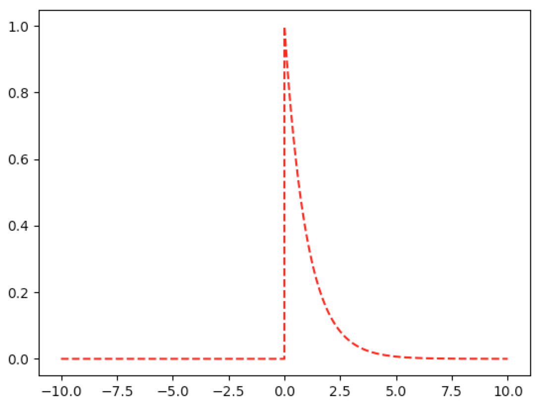
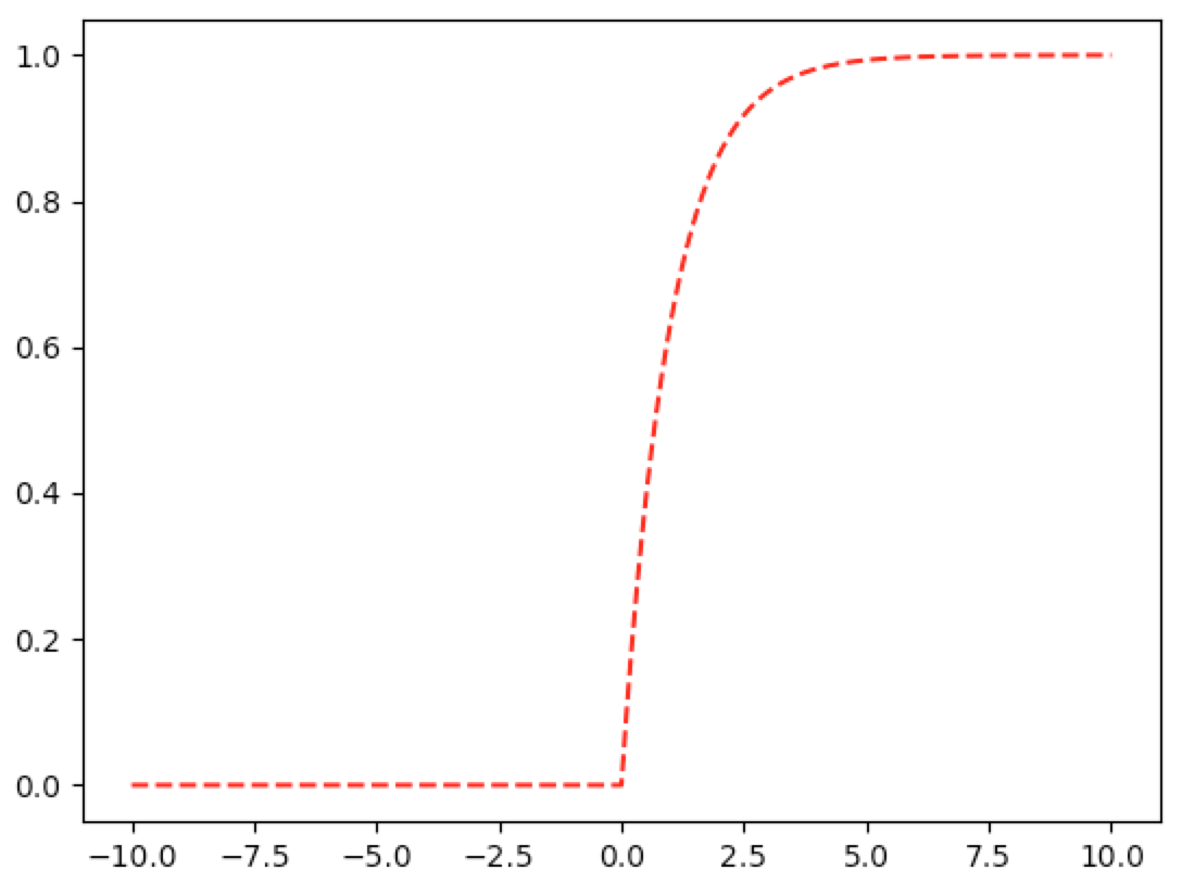
Graphs of Exponential Density and Distribution
When trying to plot these graphs, I encountered a python error that I posted to stackoverflow.
The first code snippet is the efficient approach. The second snippet is inefficient but still works.
In [1]: from numpy import exp

In [2]: from matplotlib import pyplot as plt

In [3]: import numpy as np

In [4]: def graph(funct, x_range):
   ...:     x=np.array(x_range)
   ...:     y=funct(x)
   ...:     plt.plot(x,y,'r--')
   ...:     plt.show()
   ...:

In [5]: pdf_exp=lambda x,lam=1:lam*exp(-lam*x)*(x>=0)

In [6]: cdf_exp=lambda x,lam=1:(1-exp(-lam*x))*(x>=0)

In [7]: graph(lambda x: pdf_exp(x), np.linspace(-10,10,10000))

In [8]: graph(lambda x: cdf_exp(x), np.linspace(-10,10,10000))
Inefficient Implementation:
In [1]: from numpy import exp

In [2]: from matplotlib import pyplot as plt

In [3]: def graph(funct, x_range):
   ...:     y_range=[]
   ...:     for x in x_range:
   ...:         y_range.append(funct(x))
   ...:     plt.plot(x_range,y_range,'r--')
   ...:     plt.show()
   ...:

In [4]: import numpy as np

In [5]: pdf_exp=lambda x,lam=1:lam*exp(-lam*x) if x>=0 else 0

In [6]: cdf_exp=lambda x,lam=1:1-exp(-lam*x) if x>=0 else 0

In [7]: graph(lambda x: pdf_exp(x), np.linspace(-10,10,10000))

In [8]: graph(lambda x: cdf_exp(x), np.linspace(-10,10,10000))
Poisson and Exponential, Time Estimates
Let $N_t$ denote the number of arrivals during time period $t$.
Let $X_t$ denote the time it take for one additional arrival to arrive given that someone just arrived at time $t$.
By definition, the following conditions are equivalent:
$$ X_t>x\iff N_t=N_{t+x} \tag{5.41.1} $$
To show $\implies$: if $X_t>x$, then no one arrived from time $t$ to time $t+x$. Hence $N_t=N_{t+x}$.
To show $\impliedby$: if $N_t=N_{t+x}$, then no one arrived from time $t$ to time $t+x$. Hence $X_t>x$.
Then
$$ \pr{X_t\leq x}=1-\pr{X_t>x}=1-\pr{N_{t+x}-N_t=0} $$
$$ =1-\pr{N_x=0}=1-\frac{(\lambda x)^0}{0!}\e{-\lambda x}=1-\e{-\lambda x}=F_{X_t}(x) $$
where $F_{X_t}$ is the distribution function of the the exponential random variable.
Example 5c
Let $Y$ denote the amount of time that the other person (either Ms. Jones or Mr. Brown) spends being served. Let $X$ denote the amount of time that Mr. Smith spends being served. Let $t$ denote the amount of time that Mr. Smith spends waiting to be served.
Then we wish to compare $\cp{Y>s+t}{Y>t}$ with $P(X>s)$.
$$ \cp{Y>s+t}{Y>t}=P(Y>s)=e^{-\lambda s}=P(X>s) $$
That is, the other person is just as likely as Mr. Smith to finish being served at time $s+t$. Hence both have a probability of $\frac12$ of finishing first.
The Only Memoryless Distribution Is the Exponential Distribution
Let $T$ be a continuous random variable on $[0,\infty)$. Then $T$ is memoryless if, for all $s,t\geq0$, we have:
$$ \cp{T>s+t}{T>t}=P(T>s) \tag{1} $$
By the definition of conditional probability, this is equivalent to
$$ \frac{P\set{T>s+t,T>t}}{P\set{T>t}}=P(T>s) $$
But $\set{T>s+t}$ is a subset of $\set{T>t}$, which implies that $P\set{T>s+t,T>t}=P\set{T>s+t}$. Hence (1) is equivalent to
$$ \frac{P\set{T>s+t}}{P\set{T>t}}=P(T>s) $$
or
$$ P\set{T>s+t}=P(T>s)P\set{T>t} \tag{2} $$
Proof
First recall the PDF and CDF for the exponential distribution. If $X$ is exponentially distributed, then for some $\lambda>0$, the density $f$ of $X$ is
$$ f(x)=\cases{\lambda e^{-\lambda x}&x\geq0\\0&x<0} $$
Then, for $a\geq0$, the cumulative distribution function $F$ of $X$ is
$$ F(a)=P\set{X\leq a}=\int_{0}^{a}\lambda e^{-\lambda x}dx=-e^{-\lambda x}\eval{0}{a}=e^{-\lambda0}-e^{-\lambda a}=1-e^{-\lambda a} $$
Hence $P\set{X>a}=1-\bop1-e^{-\lambda a}\bcp=e^{-\lambda a}$.
Suppose $T$ is a memoryless distribution and let $g(x)=P\set{T>x}$. Hence, to show that $T$ must be the exponential distribution, it is sufficient to show that $g(x)=e^{-\lambda x}$ for some $\lambda>0$ and for all $x\geq0$.
To this end, first note that the memoryless property of $T$ gives us
$$ \pr{T>2}=\pr{T>1+1}=\pr{T>1}\pr{T>1}=\bop\pr{T>1}\bcp^2 $$
Similarly
$$ \pr{T>3}=\pr{T>1+2}=\pr{T>1}\pr{T>2}=\pr{T>1}\bop\pr{T>1}\bcp^2=\bop\pr{T>1}\bcp^3 $$
For any positive integer $n$, an inductive argument yields
$$ \pr{T>n}=\bop\pr{T>1}\bcp^n $$
Let $\lambda=-\ln\bop\pr{T>1}\bcp$. Multiplying by $-1$ and taking the exponential of both sides, we see that $\pr{T>1}=e^{-\lambda}$ and
$$ g(n)=\pr{T>n}=\bop\pr{T>1}\bcp^n=\bop e^{-\lambda}\bcp^n=e^{-\lambda n} $$
So we have proven the desired result for the positive integers. To prove this for the positive rational numbers, note that
$$ e^{-\lambda}=\pr{T>1}=\prB{T>\frac12+\frac12}=\prB{T>\frac12}\prB{T>\frac12}=\Bop\prB{T>\frac12}\Bcp^2 $$
Hence
$$ e^{-\frac{\lambda}2}=\prB{T>\frac12} $$
Similarly, for any positive integer $m$, we have
$$ e^{-\lambda m}=\pr{T>m}=\prB{T>\frac{m}2+\frac{m}2}=\prB{T>\frac{m}2}\prB{T>\frac{m}2}=\Bop\prB{T>\frac{m}2}\Bcp^2 $$
Hence
$$ e^{-\lambda\frac{m}2}=\prB{T>\frac{m}2} $$
Similarly
$$ e^{-\lambda m}=\pr{T>m}=\prB{T>\frac{m}3+\frac{m}3+\frac{m}3}=\Bop\prB{T>\frac{m}3}\Bcp^3 $$
Hence
$$ e^{-\lambda\frac{m}3}=\prB{T>\frac{m}3} $$
An inductive argument shows that for any positive integer $n$, we have
$$ e^{-\lambda m}=\pr{T>m}=\prB{T>\sum_1^n\frac{m}n}=\Bop\prB{T>\frac{m}n}\Bcp^n $$
Hence
$$ e^{-\lambda\frac{m}n}=\prB{T>\frac{m}n}=g\Bop\frac{m}n\Bcp $$
So the desired result is proven for positive rational numbers and it suffices to prove it for positive irrational numbers. Let $t_n, n\geq1$ be a sequence of decreasing rational numbers that converge to the irrational number $t>0$. Then
$$ g(t)=\pr{T>t}=\lim_{n\goesto\infty}\pr{T>t_n}=\lim_{n\goesto\infty}e^{-\lambda t_n}=e^{-\lambda t} $$
The second equality uses the right-continuous property of the CDF.
$\wes$
Example 5d
Let $X$ denote the number of miles before the battery dies.
$$ 10K=\evw{X}=\frac1{\lambda_b}\iff\lambda_b=\frac1{10K} $$
Then $\frac{X}{1K}$ denotes the number of 1K miles before the battery dies:
$$ 10=\frac{10K}{1K}=\evwB{\frac{X}{1K}}=\frac{1}{1K\lambda_b}=\frac{1}{1K\frac1{10K}}=\frac1{\frac1{10}}=\frac1{\lambda_a}\iff\lambda_a=\frac1{10} $$
We can compute it this way
$$ \bop P(X>5K)\bcp^{2}=P(X>5K+5K) $$
$$ =P(X>10K)=1-F_b(10K)=1-\bop1-e^{-\lambda_b10K}\bcp=e^{-\lambda_b10K}=e^{-1} $$
So that
$$ P(X>5K)=\bop e^{-1}\bcp^{\frac12}=e^{-1\wts\frac12}=e^{-\frac12} $$
Or we can compute it this way
$$ P(X>5K)=1-F_b(5K)=1-\bop1-e^{-\lambda_b5K}\bcp=e^{-\lambda_b5K}=e^{-\frac1{10K}5K}=e^{-\frac12} $$
Or we can compute it this way
$$ P(X>5)=1-F_a(5)=1-\bop1-e^{-\lambda_a5}\bcp=e^{-\lambda_a5}=e^{-\frac1{10}5}=e^{-\frac12} $$
The Density Closely Approximates The Intense Probability in a Small Neighborhood
Suppose $X$ is exponentially distributed with density $f$, distribution $F$, and $\lambda>0$.
The equations at the top of p.213 assume that, for a fixed $t>0$ and any small $dt>0$, we have
$$ f(t)dt\approx\pr{X\in(t,t+dt)} $$
This is easy to picture in the $x$-$y$ plane and is equivalent to
$$ f(t)dt-\int_{t}^{t+dt}f(x)dx\approx0 $$
Here is a helpful discussion.
Rigorously we want to show that
$$ \lim_{dt\downarrow0}\Bop f(t)dt-\int_{t}^{t+dt}f(x)dx\Bcp=0 $$
This is a simple result from the definition of the Reimann Integral. But I haven’t done an $\epsilon$-$\delta$ proof in a long time. So let $\epsilon>0$. We must find $\delta>0$ such that $dt<\delta$ implies
$$ \normB{f(t)dt-\int_{t}^{t+dt}f(x)dx}<\epsilon $$
We have
$$ \normB{f(t)dt-\int_{t}^{t+dt}f(x)dx}=\normB{\lambda\e{-\lambda t}dt-\Bop-\e{-\lambda x}\eval{t}{t+dt}\Bcp} $$
$$ =\normB{\lambda\e{-\lambda t}dt+\e{-\lambda x}\eval{t}{t+dt}} $$
$$ =\normB{\lambda\e{-\lambda t}dt+\e{-\lambda t-\lambda dt}-\e{-\lambda t}} $$
$$ =\normB{\lambda\e{-\lambda t}dt+\e{-\lambda t}\e{-\lambda dt}-\e{-\lambda t}} $$
$$ =\normB{\e{-\lambda t}\bop\lambda dt+\e{-\lambda dt}-1\bcp} $$
$$ =\e{-\lambda t}\normb{\lambda dt+\e{-\lambda dt}-1} $$
$$ \leq\e{-\lambda t}\bop\norm{\lambda dt}+\norm{\e{-\lambda dt}-1}\bcp \tag{Triangle Inequality} $$
$$ =\e{-\lambda t}\bop\lambda dt+1-\e{-\lambda dt}\bcp \tag{$\lambda dt>0\implies\e{-\lambda dt}<1$} $$
$$ =\e{-\lambda t}\lambda dt+\e{-\lambda t}\bop1-\e{-\lambda dt}\bcp $$
Let’s look at the first term. We want to find $\delta_1>0$ such that $dt<\delta_1$ implies
$$ \e{-\lambda t}\lambda dt<\frac\epsilon2 $$
or
$$ dt<\frac\epsilon{2\e{-\lambda t}\lambda} $$
Set $\delta_1=\frac\epsilon{2\e{-\lambda t}\lambda}$ and we’re half way there. Now let’s look at the second term. We want to find $\delta_2>0$ such $dt<\delta_2$ implies
$$ \e{-\lambda t}\bop1-\e{-\lambda dt}\bcp<\frac\epsilon2 $$
$\iff$
$$ 1-\e{-\lambda dt}<\frac\epsilon{2\e{-\lambda t}} $$
$\iff$
$$ -\e{-\lambda dt}<\frac\epsilon{2\e{-\lambda t}}-1 $$
$\iff$
$$ \e{-\lambda dt}>1-\frac\epsilon{2\e{-\lambda t}} $$
$\iff$
$$ -\lambda dt>\ln\Bop1-\frac\epsilon{2\e{-\lambda t}}\Bcp $$
$\iff$
$$ dt<\frac{\ln\Bop1-\frac\epsilon{2\e{-\lambda t}}\Bcp}{-\lambda} $$
We note that $\frac\epsilon{2\e{-\lambda t}}>0$ so the numerator is negative and the right-hand side is positive. Set $\delta_2$ equal to the right-hand side and set $\delta=\min(\delta_1,\delta_2)$. Then $dt<\delta$ implies
$$ \normB{f(t)dt-\int_{t}^{t+dt}f(x)dx}\leq\e{-\lambda t}\lambda dt+\e{-\lambda t}\bop1-\e{-\lambda dt}\bcp<\frac\epsilon2+\frac\epsilon2=\epsilon $$
$\wes$
5.5.1 Hazard Rate Function for the Exponential Random Variable
$$ \cp{X\in(t,t+dt)}{X>t}=\frac{\pr{X\in(t,t+dt)\cap X>t}}{\pr{X>t}} $$
But $\set{X\in(t,t+dt)}\subset\set{X>t}$: Suppose $x_0\in\set{X\in(t,t+dt)}$. Then $x_0>t$ so that $x_0\in\set{X>t}$. Hence
$$ \set{X\in(t,t+dt)}\cap\set{X>t}=\set{X\in(t,t+dt)} $$
And
$$ \pr{X\in(t,t+dt)\cap X>t}=\pr{X\in(t,t+dt)} $$
And
$$ \cp{X\in(t,t+dt)}{X>t}=\frac{\pr{X\in(t,t+dt)\cap X>t}}{\pr{X>t}} $$
$$ =\frac{\pr{X\in(t,t+dt)}}{\pr{X>t}} $$
$$ =\frac{1-\pr{X\notin(t,t+dt)}}{\pr{X>t}} $$
$$ =\frac{1-\pr{X<t\cup X>t+dt}}{\pr{X>t}} $$
$$ =\frac{1-\bop\pr{X<t}+\pr{X>t+dt}\bcp}{\pr{X>t}} $$
$$ =\frac{1-\pr{X<t}-\pr{X>t+dt}}{\pr{X>t}} $$
$$ =\frac{\pr{X>t}-\pr{X>t+dt}}{\pr{X>t}} $$
$$ =1-\frac{\pr{X>t+dt}}{\pr{X>t}} $$
$$ =1-\frac{\pr{X>t}\pr{X>dt}}{\pr{X>t}} \tag{Memoryless} $$
$$ =1-\pr{X>dt} $$
$$ =\pr{X<dt} $$
In words, the memoryless property implies that the distribution of remaining life for a $t$-year-old item is the same as that for a new item. But we also have
$$ f(t)dt\approx\pr{X\in(t,t+dt)} $$
Hence
$$ \pr{X<dt}=\cp{X\in(t,t+dt)}{X>t}=\frac{\pr{X\in(t,t+dt)}}{\pr{X>t}}\approx\frac{f(t)}{\overline{F}(t)}dt=\lambda(t)dt $$
Since this holds for all $t>0$, then $\lambda(t)$ must be constant. Indeed
$$ \lambda(t)=\frac{f(t)}{\overline{F}(t)}=\frac{\lambda\e{-\lambda t}}{\e{-\lambda t}}=\lambda $$
5.5.1 Hazard Rate Function Integration
$$ \int_0^t\frac{F'(x)}{1-F(x)}dx $$
Let $u=1-F(x)$, $du=-F’(x)dx$ to get
$$ \int\frac{F'(x)}{1-F(x)}dx=\int\frac{-du}{u}=-\ln(u)+k=-\ln\bop1-F(x)\bcp+k $$
$$ \int_0^t\frac{F'(x)}{1-F(x)}dx=-\ln\bop1-F(x)\bcp\eval{0}{t}=\ln\bop1-F(x)\bcp\eval{t}{0} $$
$$ =\ln\bop1-F(0)\bcp-\ln\bop1-F(t)\bcp $$
$$ =\ln\bop1-0\bcp-\ln\bop1-F(t)\bcp \tag{since $X>0$} $$
$$ =-ln\bop1-F(t)\bcp $$
Example 6a Expectation and Variance of Gamma Random Variable
$$ \evw{X}=\frac1{\GammaF{\alpha}}\int_0^\infty x\lambda\e{-\lambda x}(\lambda x)^{\alpha-1}dx $$
$$ =\frac1{\GammaF{\alpha}}\int_0^\infty\frac{\lambda x}\lambda\lambda\e{-\lambda x}(\lambda x)^{\alpha-1}dx $$
$$ =\frac1{\lambda\GammaF{\alpha}}\int_0^\infty\lambda\e{-\lambda x}(\lambda x)^{\alpha}dx \tag{5.6a.1} $$
We want to show that
$$ \int_0^\infty\lambda\e{-\lambda x}(\lambda x)^{\alpha}dx=\GammaF{\alpha+1} $$
The substitution $y=\lambda x$ gives us
$$ x=\frac{y}\lambda\dq dx=\frac{dy}{\lambda}\dq y_0=\lambda x_0=0\dq y_1=\lambda x_1=\infty $$
$$ \int_0^\infty\lambda\e{-\lambda x}(\lambda x)^{\alpha}dx=\int_0^\infty\lambda\e{-y}y^\alpha\frac{dy}\lambda=\int_0^\infty\e{-y}y^{\alpha}dy=\GammaF{\alpha+1} $$
Hence 5.6a.1 becomes
$$ \evw{X}=\frac{\GammaF{\alpha+1}}{\lambda\GammaF{\alpha}}=\frac\alpha\lambda $$
where the last equation follows from equation 6.1 in the book.
Next we want to find $\varw{X}$:
$$ \evwb{X^2}=\frac1{\GammaF{\alpha}}\int_0^\infty x^2\lambda\e{-\lambda x}(\lambda x)^{\alpha-1}dx $$
The substitution $y=\lambda x$ gives us
$$ x=\frac{y}\lambda\dq dx=\frac{dy}{\lambda}\dq y_0=\lambda x_0=0\dq y_1=\lambda x_1=\infty $$
$$ \evwb{X^2}=\frac1{\GammaF{\alpha}}\int_0^\infty\Prn{\frac{y}{\lambda}}^2\lambda\e{-y}y^{\alpha-1}\frac{dy}\lambda $$
$$ =\frac1{\GammaF{\alpha}}\int_0^\infty\Prn{\frac{y}{\lambda}}^2\e{-y}y^{\alpha-1}dy $$
$$ =\frac1{\lambda^2\GammaF{\alpha}}\int_0^\infty y^2\e{-y}y^{\alpha-1}dy $$
$$ =\frac1{\lambda^2\GammaF{\alpha}}\int_0^\infty\e{-y}y^{\alpha+1}dy $$
$$ =\frac{\GammaF{\alpha+2}}{\lambda^2\GammaF{\alpha}}=\frac{(\alpha+1)\GammaF{\alpha+1}}{\lambda^2\GammaF{\alpha}}=\frac{(\alpha+1)\alpha\GammaF{\alpha}}{\lambda^2\GammaF{\alpha}} $$
$$ =\frac{\alpha(\alpha+1)}{\lambda^2} $$
And
$$ \varw{X}=\frac{\alpha(\alpha+1)}{\lambda^2}-\Prn{\frac\alpha\lambda}^2=\frac{\alpha(\alpha+1)-\alpha^2}{\lambda^2}=\frac{\alpha^2+\alpha-\alpha^2}{\lambda^2}=\frac\alpha{\lambda^2} $$
Example 7b
$$ \cdfa{y}{Y}=\cdfa{\sqrt{y}}{X}-\cdfa{-\sqrt{y}}{X} $$
Then the density is
$$ \pdfa{y}{Y}=\wderiv{\cdfu{Y}}{y}=\wderiv{\cdfu{X}}{\sqrt{y}}\wderiv{\sqrt{y}}{y}-\wderiv{\cdfu{X}}{(-\sqrt{y})}\wderiv{(-\sqrt{y})}{y} $$
$$ =\pdfa{\sqrt{y}}{X}\frac12y^{-\frac12}-\pdfa{-\sqrt{y}}{X}\prn{-\frac12y^{-\frac12}} $$
$$ =\pdfa{\sqrt{y}}{X}\frac1{2\sqrt{y}}+\pdfa{-\sqrt{y}}{X}\frac1{2\sqrt{y}} $$
Succintly, we have
$$ \pdfa{y}{Y}=\frac1{2\sqrt{y}}\prn{\pdfa{\sqrt{y}}{X}+\pdfa{-\sqrt{y}}{X}} \tag{5.7b.1} $$
Now let’s try applying Theorem 7.1 to this problem and check that it agrees with 5.7b.1. Further suppose that $X$ is nonnegative. Define $g(x)\equiv x^2$. Since $X$ is nonnegative, then $g(\wt)$ is strictly increasing on the range of $X$ and hence is invertible:
$$ \inv{g}(y)=\sqrt{y}=y^{\frac12} $$
And the derivative of the inverse is
$$ \wdervb{y}{\inv{g}(y)}=\frac12y^{-\frac12}=\frac1{2\sqrt{y}}>0 $$
And
$$ \normB{\wdervb{y}{\inv{g}(y)}}=\wdervb{y}{\inv{g}(y)} $$
Also note that for every $y\geq0$, there exists $x\geq0$ such that $y=g(x)$. Namely, set $x=\sqrt{y}$. Then $g(x)=g\prn{\sqrt{y}}=\prn{\sqrt{y}}^2=y$. Hence for $y\geq0$ we have
$$ \pdfa{y}{Y}=\pdfab{\inv{g}(y)}{X}\normB{\wdervb{y}{\inv{g}(y)}}=\pdfa{\sqrt{y}}{X}\frac1{2\sqrt{y}} $$
Also note that since $X$ is nonnegative, we have $\pdfa{-\sqrt{y}}{X}=0$. Hence
$$ \pdfa{y}{Y}=\frac1{2\sqrt{y}}\pdfa{\sqrt{y}}{X}=\frac1{2\sqrt{y}}\prn{\pdfa{\sqrt{y}}{X}+0}=\frac1{2\sqrt{y}}\prn{\pdfa{\sqrt{y}}{X}+\pdfa{-\sqrt{y}}{X}} $$
This agrees with 5.7b.1 above.
Theorem 7.1
I have some intuition on the statement “When $y\neq g(x)$ for any $x$, then $\cdfa{y}{Y}$ is either $0$ or $1$, an in either case $\pdfa{y}{Y}=0$”. But I’d like to see an example.
We’ll use the exponential distribution:
$$ \pdf{x}=\cases{\lambda\e{-\lambda x}&x\geq0\\0&x<0} $$
And $Y=X^2$ is increasing on the range of $X$, which is $[0,\infty)$. Let’s look at $Y=-7$. There’s no $X$ value such that $-7=X^2$. We know from example 7b above that
$$ \pdfa{y}{Y}=\cases{\frac1{2\sqrt{y}}\pdf{\sqrt{y}}&y\geq0\\0&y<0} $$
Or
$$ \pdfa{y}{Y}=\cases{\frac{\lambda\e{-\lambda\sqrt{y}}}{2\sqrt{y}}&y\geq0\\0&y<0} $$
Hence $\pdfa{-7}{Y}=0$ is verified for this example.