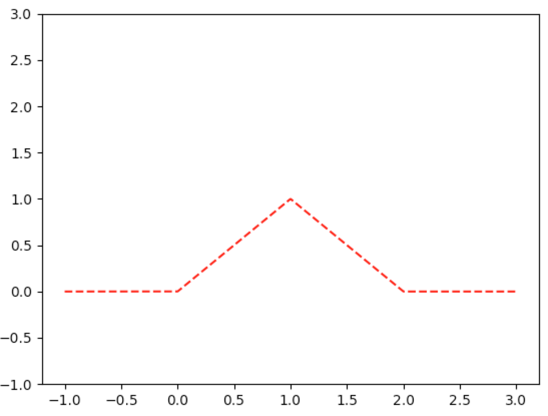
Example 3a
$$ \pdfa{a}{X+Y}=\int_0^1\pdfa{a-y}{X}dy $$
$$ x=a-y\dq y=a-x\dq dy=-dx\dq x_0=a-y_0=a\dq x_1=a-y_1=a-1 $$
$$ \pdfa{a}{X+Y}=-\int_a^{a-1}\pdfa{x}{X}dx=\int_{a-1}^a\pdfa{x}{X}dx=\cdfa{x}{X}\eval{a-1}{a} $$
In [1]: from numpy import exp

In [2]: from matplotlib import pyplot as plt

In [3]: import numpy as np

In [4]: def graph(funct, x_range):
   ...:     x=np.array(x_range)
   ...:     y=funct(x)
   ...:     plt.plot(x,y,'r--')
   ...:     plt.show()
   ...:

In [5]: def graph_ineff(funct, x_range):
   ...:     y_range=[]
   ...:     for x in x_range:
   ...:         y_range.append(funct(x))
   ...:     plt.plot(x_range,y_range,'r--')
   ...:     plt.show()
   ...:

In [6]: plt.ylim(-1,3)
Out[6]: (-1, 3)

In [7]: cdf_unif=lambda x=1:0 if x<=0 else x if x<=1 else 1

In [8]: graph_ineff(lambda x: cdf_unif(x)-cdf_unif(x-1), np.linspace(-1,3,1000))
Integral Compute - Bottom of p.253
$$ \frac1{(n-1)!}\int_0^x(x-y)^{n-1}dy $$
$$ u=x-y\dq y=x-u\dq dy=-du\dq u_0=x-y_0=x\dq u_1=x-y_1=0 $$
$$ \frac1{(n-1)!}\int_0^x(x-y)^{n-1}dy=-\frac1{(n-1)!}\int_x^0u^{n-1}du=\frac1{(n-1)!}\int_0^xu^{n-1}du $$
$$ =\frac1{(n-1)!}\frac{u^n}{n}\eval{0}{x}=\frac1{n!}\prn{x^n-0^n}=\frac{x^n}{n!} $$
Compute - Top of p.254
$$ \pr{N=n}=\pr{N\leq n}-\pr{N<n} $$
$$ =1-\pr{N>n}-\pr{N\leq n-1} $$
$$ =1-\pr{N>n}-\prn{1-\pr{N>n-1}} $$
$$ =1-\pr{N>n}-1+\pr{N>n-1} $$
$$ =\pr{N>n-1}-\pr{N>n} $$
Also:
$$ \evw{N}=\sum_{n=1}^{\infty}\frac{n(n-1)}{n!} $$
$$ =\frac{1\wts(1-1)}{1!}+\sum_{n=2}^{\infty}\frac{n(n-1)}{n!} $$
$$ =\frac{1\wts0}{1!}+\sum_{n=2}^{\infty}\frac{1}{(n-2)!} $$
$$ =\sum_{n=2}^{\infty}\frac{1}{(n-2)!} $$
In [22]: sum([1/wf(i-2) for i in range(2,20)])
Out[22]: 2.7182818284590455
Proposition 3.1
$$ \pdf{y}=\frac{\lambda\e{-\lambda y}(\lambda y)^{t-1}}{\GammaF{t}}\dq0<y<\infty $$
Closed under convolutions:
$$ \pdfa{a}{X+Y}=\int_{-\infty}^{\infty}\pdfa{a-y}{X}\pdfa{y}{Y}dy \tag{Eq 3.2, p.252} $$
$$ =\int_{0}^{a}\pdfa{a-y}{X}\pdfa{y}{Y}dy \tag{P.3.1.1} $$
$$ =\frac1{\GammaF{s}\GammaF{t}}\int_{0}^{a}\lambda\e{-\lambda(a-y)}[\lambda(a-y)]^{s-1}\lambda\e{-\lambda y}(\lambda y)^{t-1}dy $$
$$ =\frac1{\GammaF{s}\GammaF{t}}\int_{0}^{a}\lambda\e{-\lambda a}\e{\lambda y}\e{-\lambda y}[\lambda(a-y)]^{s-1}\lambda(\lambda y)^{t-1}dy $$
$$ =\frac{\e{-\lambda a}}{\GammaF{s}\GammaF{t}}\int_{0}^{a}\lambda[\lambda(a-y)]^{s-1}\lambda(\lambda y)^{t-1}dy $$
$$ =\frac{\lambda^2\lambda^{s-1}\lambda^{t-1}\e{-\lambda a}}{\GammaF{s}\GammaF{t}}\int_{0}^{a}(a-y)^{s-1}y^{t-1}dy $$
$$ =\frac{\lambda^{s+t}\e{-\lambda a}}{\GammaF{s}\GammaF{t}}\int_{0}^{a}(a-y)^{s-1}y^{t-1}dy \tag{P.3.1.2} $$
Eq. P.3.1.1 follows because the Gamma density is zero for negative values. So $\pdfa{y}{Y}=0$ when $y<0$. And $\pdfa{a-y}{X}=0$ when $y>a$.
Now let’s look at the integral in Eq. P.3.1.2.
$$ x=\frac{y}{a}\dq y=ax\dq dy=adx\dq x_0=\frac{y_0}{a}=0\dq x_1=\frac{y_1}{a}=1 $$
$$ \int_{0}^{a}(a-y)^{s-1}y^{t-1}dy=\int_{0}^{a}\Sbr{a\Prn{1-\frac{y}{a}}}^{s-1}y^{t-1}dy $$
$$ =\int_{0}^{1}[a(1-x)]^{s-1}(ax)^{t-1}adx $$
$$ =\int_{0}^{1}a^{s-1}(1-x)^{s-1}a^{t-1}x^{t-1}adx $$
$$ =a^{s-1}a^{t-1}a\int_{0}^{1}(1-x)^{s-1}x^{t-1}dx $$
$$ =a^{s+t-1}\int_{0}^{1}(1-x)^{s-1}x^{t-1}dx $$
$$ =a^{s+t-1}\frac{\GammaF{s}\GammaF{t}}{\GammaF{s+t}} $$
The last equality (Beta and Gamma relationship) follows from equation 6.3 on p.218. On page p.219, the author claims verification of eq. 6.3 occurs in Example 7c of Ch.6. We’ll see.
Hence Eq. P.3.1.2 becomes
$$ \pdfa{a}{X+Y}=\frac{\lambda^{s+t}\e{-\lambda a}}{\GammaF{s}\GammaF{t}}a^{s+t-1}\frac{\GammaF{s}\GammaF{t}}{\GammaF{s+t}} $$
$$ =\frac{\lambda^{s+t}\e{-\lambda a}a^{s+t-1}}{\GammaF{s+t}} $$
$$ =\frac{\lambda\lambda^{s+t-1}\e{-\lambda a}a^{s+t-1}}{\GammaF{s+t}} $$
$$ =\frac{\lambda\e{-\lambda a}(\lambda a)^{s+t-1}}{\GammaF{s+t}} $$
Hence $X+Y$ is a Gamma random variable with parameters $(s + t, λ)$.
$\wes$
Compute - Middle of p.255
The standard normal density is
$$ \pdfa{y}{Z}=\frac1{\sqrt{2\pi}}\e{-\frac{y^2}2} $$
Hence
$$ \pdfa{y}{Z^2}=\frac1{2\sqrt{y}}\sbr{\pdfa{\sqrt{y}}{Z}+\pdfa{-\sqrt{y}}{Z}} $$
$$ =\frac1{2\sqrt{y}}\Sbr{\frac1{\sqrt{2\pi}}\e{-\frac{y}2}+\frac1{\sqrt{2\pi}}\e{-\frac{y}2}} $$
$$ =\frac1{2\sqrt{y}}\frac2{\sqrt{2\pi}}\e{-\frac{y}2} $$
$$ =\frac{\e{-\frac{y}2}}{\sqrt{y}\sqrt{2\pi}}=\frac{\e{-\frac{y}2}\sqrt{2}}{2\sqrt{y}\sqrt{\pi}}=\frac{\e{-\frac{y}2}y^{-\frac12}2^{\frac12}}{2\sqrt{\pi}}=\frac{\e{-\frac{y}2}y^{-\frac12}\prn{\frac12}^{-\frac12}}{2\sqrt{\pi}} $$
$$ =\frac{\e{-\frac{y}2}\prn{\frac{y}2}^{-\frac12}}{2\sqrt{\pi}}=\frac{\frac12\e{-\frac{y}2}\prn{\frac{y}2}^{\frac12-1}}{\sqrt{\pi}} $$
Example 3d
$$ \prB{Z>\frac{-0.0165}{0.0730}}=1-\prB{Z<\frac{-0.0165}{0.0730}} $$
$$ =1-\Prn{1-\prB{Z<\frac{0.0165}{0.0730}}} $$
$$ =\prB{Z<\frac{0.0165}{0.0730}} $$
In [32]: phi(.0165/.073)
Out[32]: 0.58940994413412728
We can talk about conditional distributions when the random variables are neither jointly continuous nor jointly discrete. For example, suppose that $X$ is a continuous random variable having probability density function $f$. Also suppose that $N$ is a discrete random variable, and consider the conditional distribution of $X$ given that $N=n$. We wish to show that
$$ \pdfa{x|n}{X|N}=\frac{\cp{N=n}{X=x}}{\pr{N=n}}\pdf{x} $$
Note that
$$ \frac{\cp{x<X<x+dx}{N=n}}{dx}=\frac{\pr{x<X<x+dx,N=n}}{\pr{N=n}}\frac1{dx} $$
$$ =\frac{\cp{N=n}{x<X<x+dx}}{\pr{N=n}}\frac{\pr{x<X<x+dx}}{dx} $$
So that
$$ \lim_{dx\goesto0}\frac{\cp{x<X<x+dx}{N=n}}{dx} $$
$$ =\lim_{dx\goesto0}\Cbr{\frac{\cp{N=n}{x<X<x+dx}}{\pr{N=n}}\frac{\pr{x<X<x+dx}}{dx}} $$
$$ =\frac{\lim_{dx\goesto0}\cp{N=n}{x<X<x+dx}}{\pr{N=n}}\lim_{dx\goesto0}\frac{\pr{x<X<x+dx}}{dx} \tag{T.p.268.1} $$
Apparently we can take the limit of the given event inside the conditional probability:
$$ \lim_{dx\goesto0}\cp{N=n}{x<X<x+dx}=\cp{N=n}{X=x} $$
Let $\prq{\wt}=\cp{\wt}{N=n}$. Then $Q$ is a probability function:
$$ \lim_{dx\goesto0}\cp{N=n}{x<X<x+dx}=\lim_{dx\goesto0}\frac{\cp{x<X<x+dx}{N=n}\pr{N=n}}{\pr{x<X<x+dx}} \tag{Bayes} $$
$$ =\pr{N=n}\lim_{dx\goesto0}\frac{\prq{x<X<x+dx}}{\pr{x<X<x+dx}} $$
$$ =\pr{N=n}\lim_{dx\goesto0}\frac{\prq{X<x+dx}-\prq{X<x}}{\pr{X<x+dx}-\pr{X<x}} $$
Now the numerator and denominator each go to zero. Use L’hopital’s Rule somehow?????
Also note that
$$ \pdf{x}=\wderiv{F}{x}(x)=\lim_{dx\goesto0}\frac{\cdf{x+dx}-\cdf{x}}{dx} $$
$$ =\lim_{dx\goesto0}\frac{\pr{X<x+dx}-\pr{X<x}}{dx} $$
$$ =\lim_{dx\goesto0}\frac{\pr{x<X<x+dx}}{dx} $$
Similarly we have
$$ \pdfa{x|n}{X|N}=\wdervb{x}{\cdfa{x|n}{X|N}}=\lim_{dx\goesto0}\frac{\cdfa{x+dx|n}{X|N}-\cdfa{x|n}{X|N}}{dx} $$
$$ =\lim_{dx\goesto0}\frac{\cp{X<x+dx}{N=n}-\cp{X<x}{N=n}}{dx} $$
$$ =\lim_{dx\goesto0}\frac{\cp{x<X<x+dx}{N=n}}{dx} $$
So Eq. T.p.268.1 becomes
$$ \pdfa{x|n}{X|N}=\lim_{dx\goesto0}\frac{\cp{x<X<x+dx}{N=n}}{dx}=\frac{\cp{N=n}{X=x}}{\pr{N=n}}\pdf{x} \tag{T.p.268.2} $$
Example 5d p.269-270
Consider $n+m$ trials having a common probability of success. Suppose, however, that this success probability is not fixed in advance but is chosen from a uniform $(0, 1)$ population. What is the conditional distribution of the success probability given that the $n+m$ trials result in $n$ successes?
Solution: If we let $X$ denote the probability that a given trial is a success, then $X$ is a uniform (0, 1) random variable. Also, given that $X=x$, the $n+m$ trials are independent with common probability of success $x$, so $N$, the number of successes, is a binomial random variable with parameters $(n+m,x)$. Hence, the conditional density of $X$ given that $N=n$ is
$$ \pdfa{x|n}{X|N}=\frac{\cp{N=n}{X=x}\wts\pdfa{x}{X}}{\pr{N=n}} \tag{From T.p.268.2} $$
$$ =\frac{\binom{n+m}{n}x^n(1-x)^m\wts1}{\pr{N=n}} \tag{6.5d.1} $$
Note that
$$ \pr{N=n}=\frac1{n+m+1} $$
This is true since there are $n+m+1$ equally-likely possible success counts: $0,1,…,n+m-1,n+m$. Hence
$$ \frac{\binom{n+m}{n}}{\pr{N=n}}=\frac{\frac{(n+m)!}{n!m!}}{\frac1{n+m+1}}=\frac{(n+m+1)(n+m)!}{n!m!}=\frac{\GammaF{n+m+2}}{\GammaF{n+1}\GammaF{m+1}} $$
So Eq. 6.5d.1 becomes
$$ \pdfa{x|n}{X|N}=\frac{\GammaF{n+m+2}}{\GammaF{n+1}\GammaF{m+1}}x^n(1-x)^m $$
This matches with the discussion of the Beta distribution with Gamma coefficients in section 5.6.4.
Example 6a p.271-272
Let’s consider the joint inequalities: $X_{(3)}>X_{(2)}+d,X_{(2)}>X_{(1)}+d$. For both to be true, two conditions must be true: $X_{(1)}\leq1-2d$ and $X_{(2)}\leq1-d$. Suppose $X_{(2)}>1-d$. Then $1<X_{(2)}+d<X_{(3)}$. But it was given that $X_{(3)}\leq1$, contradiction. Similarly, suppose $X_{(1)}>1-2d$. Then $1<X_{(1)}+2d<X_{(2)}+d<X_{(3)}$. But it was given that $X_{(3)}\leq1$, contradiction.
This is easy to picture geometrically with a numerical value for $d$. Suppose $d=\frac49$. If $X_{(2)}>1-\frac49=\frac59$, then
$$ X_{(3)}>X_{(2)}+\frac49>\frac59+\frac49=1 $$
Similarly, if $X_{(1)}>1-2\wts\frac49=1-\frac89=\frac19$, then
$$ X_{(3)}>X_{(2)}+\frac49>X_{(1)}+2\wts\frac49>\frac19+\frac89=1 $$
Hence
$$ \pr{X_{(3)}>X_{(2)}+d,X_{(2)}>X_{(1)}+d}=\iiint_{\substack{x_3>x_2+d\\1-d\geq x_2>x_1+d\\1-2d\geq x_1}}\pdfa{x_1,x_2,x_3}{X_{(1)},X_{(2)},X_{(3)}}dx_1dx_2dx_3 $$
$$ =3!\int_{0}^{1-2d}\int_{x_1+d}^{1-d}\int_{x_2+d}^{1}dx_3dx_2dx_1 $$
$$ =6\int_{0}^{1-2d}\int_{x_1+d}^{1-d}(1-d-x_2)dx_2dx_1 $$
$$ y_2=1-d-x_2\dq x_2=1-d-y_2\dq dx_2=-dy_2 $$
$$ y_2^{(0)}=1-d-x_2^{(0)}=1-d-(x_1+d)=1-2d-x_1 $$
$$ y_2^{(1)}=1-d-x_2^{(1)}=1-d-(1-d)=0 $$
$$ =6\int_{0}^{1-2d}\int_{1-2d-x_1}^{0}-y_2dy_2dx_1 $$
$$ =6\int_{0}^{1-2d}\int_{0}^{1-2d-x_1}y_2dy_2dx_1 $$
$$ =6\int_{0}^{1-2d}\Sbr{\frac{y_2^2}2\eval{0}{1-2d-x_1}}dx_1 $$
$$ =6\wts\frac12\wts\int_{0}^{1-2d}\Sbr{y_2^2\eval{0}{1-2d-x_1}}dx_1 $$
$$ =3\int_{0}^{1-2d}\sbr{1-2d-x_1}^2dx_1 $$
$$ y_1=1-2d-x_1\dq x_1=1-2d-y_1\dq dx_1=-dy_1 $$
$$ y_1^{(0)}=1-2d-x_1^{(0)}=1-2d-0=1-2d $$
$$ y_1^{(1)}=1-2d-x_1^{(1)}=1-2d-(1-2d)=0 $$
$$ =3\int_{1-2d}^{0}-y_1^2dy_1 $$
$$ =3\int_{0}^{1-2d}y_1^2dy_1 $$
$$ =3\Sbr{\frac{y_1^3}3\eval{0}{1-2d}}=y_1^3\eval0{1-2d}=(1-2d)^3 $$
Example 7b p.276-277
Let $(X,Y)$ denote a random point in the plane, and assume that the rectangular coordinates $X$ and $Y$ are independent standard normal random variables. We are interested in the joint distribution of $R,\Theta$, the polar coordinate representation of $(x,y)$.
Suppose first that $X$ and $Y$ are both positive. For $x$ and $y$ positive, letting $r=g_1(x,y)=\sqrt{x^2+y^2}$ and $\theta=g_2(x,y)=\inv{\tan}\fracpb{y}{x}$, we see that
$$ \wpart{g_1}{x}=\frac12\frac1{\sqrt{x^2+y^2}}2x=\frac{x}{\sqrt{x^2+y^2}} $$
$$ \wpart{g_1}{y}=\frac{y}{\sqrt{x^2+y^2}} $$
Derivative of the arctan by MIT OCW
$$ \wpart{g_2}{x}=\frac1{1+\fracpb{y}{x}^2}\fracpB{-y}{x^2}=\frac{-y}{x^2+y^2} $$
$$ \wpart{g_2}{y}=\frac1{1+\fracpb{y}{x}^2}\fracpB{1}{x}=\frac{x}{x^2+y^2} $$
Hence
$$ J(x,y)=\vmtrx{\frac{x}{\sqrt{x^2+y^2}}&\frac{y}{\sqrt{x^2+y^2}}\\\frac{-y}{x^2+y^2}&\frac{x}{x^2+y^2}} \tag{6.7b.0} $$
$$ =\frac{x}{\sqrt{x^2+y^2}}\frac{x}{x^2+y^2}-\frac{y}{\sqrt{x^2+y^2}}\frac{-y}{x^2+y^2} $$
$$ =\frac{x^2}{(x^2+y^2)^\frac32}+\frac{y^2}{(x^2+y^2)^\frac32} $$
$$ =\frac{x^2+y^2}{(x^2+y^2)^\frac32}=\frac{1}{(x^2+y^2)^\frac12}=\frac1r $$
Aside: for continuous random variables $A$ and $B$, recall the conditional density of $A$ given that $B=b$:
$$ \pdfa{a|b}{A|B}=\frac{\pdf{a,b}}{\pdfa{b}{B}} \tag{Section 6.5, p.266} $$
I guess I can see where this translates to the conditional joint density function of $X,Y$ given that they are both positive:
$$ \pdf{x,y|X>0,Y>0}=\frac{\pdf{x,y}}{\pr{X>0,Y>0}} $$
$$ =\frac{\pdfa{x}{X}\pdfa{y}{Y}}{\pr{X>0}\pr{Y>0}} \tag{Assumed independence} $$
$$ =\frac{\frac1{\sqrt{2\pi}}\e{-\frac{x^2}2}\frac1{\sqrt{2\pi}}\e{-\frac{y^2}2}}{\frac12\frac12} $$
$$ =4\wts\frac1{2\pi}\e{-\frac{x^2+y^2}2}=\frac2{\pi}\e{-\frac{x^2+y^2}2}\dq x>0,y>0 $$
Then the conditional joint density of $R=\sqrt{X^2+Y^2}$ and $\Theta=\inv{\tan}\fracpb{Y}{X}$, given that $X$ and $Y$ are positive, is
$$ \pdfa{r,\theta|X>0,Y>0}{R,\Theta}=\pdfa{x,y|X>0,Y>0}{X,Y}\inv{\normb{J(x,y)}} $$
$$ =\cases{\frac2\pi r\e{-\frac{r^2}{2}}&0<\theta<\frac\pi2,0<r<\infty\\0&\text{otherwise}} $$
We can similarly show that
$$ \pdfa{r,\theta|X<0,Y>0}{R,\Theta}=\cases{\frac2\pi r\e{-\frac{r^2}{2}}&\frac\pi2<\theta<\pi,0<r<\infty\\0&\text{otherwise}} $$
$$ \pdfa{r,\theta|X<0,Y<0}{R,\Theta}=\cases{\frac2\pi r\e{-\frac{r^2}{2}}&\pi<\theta<\frac{3\pi}2,0<r<\infty\\0&\text{otherwise}} $$
$$ \pdfa{r,\theta|X>0,Y<0}{R,\Theta}=\cases{\frac2\pi r\e{-\frac{r^2}{2}}&\frac{3\pi}2<\theta<2\pi,0<r<\infty\\0&\text{otherwise}} $$
And now we condition the joint density of $R,\Theta$ by giving equal weights to each of these $4$ conditional joint densities:
$$ \pdfa{r,\theta}{R,\Theta}=\frac14\pdfa{r,\theta|X>0,Y>0}{R,\Theta}+\frac14\pdfa{r,\theta|X<0,Y>0}{R,\Theta} $$
$$ +\frac14\pdfa{r,\theta|X<0,Y<0}{R,\Theta}+\frac14\pdfa{r,\theta|X>0,Y<0}{R,\Theta} $$
$$ =\cases{\frac14\frac2\pi r\e{-\frac{r^2}2}&0<\theta<\frac\pi2,0<r<\infty\\\frac14\frac2\pi r\e{-\frac{r^2}2}&\frac\pi2<\theta<\pi,0<r<\infty\\\frac14\frac2\pi r\e{-\frac{r^2}2}&\pi<\theta<\frac{3\pi}2,0<r<\infty\\\frac14\frac2\pi r\e{-\frac{r^2}2}&\frac{3\pi}2<\theta<2\pi,0<r<\infty} $$
$$ =\frac1{2\pi}r\e{-\frac{r^2}2}\dq 0<\theta<2\pi,0<r<\infty $$
Now, this joint density factors into the marginal densities for $R$ and $\Theta$, so, by Proposition 2.1, p.245 (as well as the discussion on p.241), $R$ and $\Theta$ are independent random variables, with $\Theta$ being uniformly distributed over $(0,2\pi)$ and $R$ having the Rayleigh distribution with density
$$ \pdf{r}=r\e{-\frac{r^2}2}\dq 0<\theta<2\pi,0<r<\infty $$
For instance, when one is aiming at a target in the plane, if the horizontal and vertical miss distances are independent standard normals, then the absolute value of the error has the preceding Rayleigh distribution.
This result is quite interesting, for it certainly is not evident a priori that a random vector whose coordinates are independent standard normal random variables will have an angle of orientation that not only is uniformly distributed, but also is independent of the vector’s distance from the origin.
Now suppose we want the joint distribution of $R^2$ and $Θ$. Set the transformation $d=g_1(x,y)=x^2+y^2$ and $\theta=g_2(x,y)=\inv{\tan}\fracpb{y}{x}$. This transformation has the Jacobian
$$ J(x,y)=\vmtrx{2x&2y\\\frac{-y}{x^2+y^2}&\frac{x}{x^2+y^2}} \tag{Similar to 6.7b.0} $$
$$ =\frac{2x^2}{x^2+y^2}-\frac{-2y^2}{x^2+y^2} $$
$$ =\frac{2x^2+2y^2}{x^2+y^2}=\frac{2(x^2+y^2)}{x^2+y^2}=2 $$
Hence
$$ \pdfa{d,\theta|X>0,Y>0}{R^2,\Theta}=\pdfa{x,y|X>0,Y>0}{X,Y}\inv{\normb{J(x,y)}} $$
$$ =\cases{\frac2\pi\frac12\e{-\frac{d}{2}}&0<\theta<\frac\pi2,0<d<\infty\\0&\text{otherwise}} $$
and similarly for the other intervals $\theta\in(\frac\pi2,\pi),\theta\in(\pi,\frac{3\pi}2),\theta\in(\frac{3\pi}{2},2\pi)$. And in the same way as we averaged the conditional densities above with equal weights of $\frac14$, we arrive at
$$ \pdfa{d,\theta}{R^2,\Theta}=\cases{\frac14\frac1\pi\e{-\frac{d}2}&0<\theta<\frac\pi2,0<d<\infty\\\frac14\frac1\pi\e{-\frac{d}2}&\frac\pi2<\theta<\pi,0<d<\infty\\\frac14\frac1\pi\e{-\frac{d}2}&\pi<\theta<\frac{3\pi}2,0<d<\infty\\\frac14\frac1\pi\e{-\frac{d}2}&\frac{3\pi}2<\theta<2\pi,0<d<\infty} $$
$$ =\frac1{2\pi}\frac12\e{-\frac{d}2}\dq 0<\theta<2\pi,0<d<\infty $$
Therefore, $R^2$ and $\Theta$ are independent, with $R^2$ having an exponential distribution with parameter $\frac12$. But because $R^2=X^2+Y^2$, it follows by definition that $R^2$ has a chi-squared distribution with $2$ degrees of freedom. Hence, we have a verification of the result that the exponential distribution with parameter $\frac12$ is the same as the chi-squared distribution with $2$ degrees of freedom.
Box-Muller p.278
$$ X_1=\sqrt{-2\log{U_1}}\cos(2\pi U_2) \tag{6.7b.1} $$
$$ X_2=\sqrt{-2\log{U_1}}\sin(2\pi U_2) \tag{6.7b.2} $$
First we want to find the inverses:
$$ X_1^2=-2\log{U_1}\cos^2(2\pi U_2) $$
$$ X_2^2=-2\log{U_1}\sin^2(2\pi U_2) $$
$\iff$
$$ \e{-\frac12X_1^2}=\e{\log{U_1}\cos^2(2\pi U_2)} $$
$$ \e{-\frac12X_2^2}=\e{\log{U_1}\sin^2(2\pi U_2)} $$
$\iff$
$$ \e{-\frac12X_1^2}\e{-\frac12X_2^2}=\e{\log{U_1}\cos^2(2\pi U_2)}\e{\log{U_1}\sin^2(2\pi U_2)} $$
$\iff$
$$ \e{-\frac12X_1^2-\frac12X_2^2}=\e{\log{U_1}\cos^2(2\pi U_2)+\log{U_1}\sin^2(2\pi U_2)} $$
$\iff$
$$ \e{-\frac12(X_1^2+X_2^2)}=\e{\log{U_1}[\cos^2(2\pi U_2)+\sin^2(2\pi U_2)]}=\e{\log{U_1}\wts1}=U_1 $$
Dividing 6.7b.1 into 6.7b.2, we get
$$ \frac{X_2}{X_1}=\frac{\sin(2\pi U_2)}{\cos(2\pi U_2)}=\tan(2\pi U_2) $$
$\iff$
$$ \inv{\tan}\Prn{\frac{X_2}{X_1}}=2\pi U_2 $$
Succintly, we have
$$ U_1=\e{-\frac12(X_1^2+X_2^2)}\dq U_2=\frac1{2\pi}\inv{\tan}\Prn{\frac{X_2}{X_1}} \tag{6.7b.3} $$
Let’s compute the Jacobian:
$$ \wpart{X_1}{u_1}=\frac12\frac{\cos(2\pi u_2)}{\sqrt{-2\log{u_1}}}\frac{-2}{u_1}=-\frac{\cos(2\pi u_2)}{u_1\sqrt{-2\log{u_1}}} $$
$$ \wpart{X_1}{u_2}=-2\pi\sqrt{-2\log{u_1}}\sin(2\pi u_2) $$
$$ \wpart{X_2}{u_1}=-\frac{\sin(2\pi u_2)}{u_1\sqrt{-2\log{u_1}}} $$
$$ \wpart{X_2}{u_2}=2\pi\sqrt{-2\log{u_1}}\cos(2\pi u_2) $$
$$ J(u_1,u_2)=\vmtrx{-\frac{\cos(2\pi u_2)}{u_1\sqrt{-2\log{u_1}}}&-2\pi\sqrt{-2\log{u_1}}\sin(2\pi u_2)\\-\frac{\sin(2\pi u_2)}{u_1\sqrt{-2\log{u_1}}}&2\pi\sqrt{-2\log{u_1}}\cos(2\pi u_2)} $$
$$ =-\frac{2\pi}{u_1}\cos^2(2\pi u_2)-\frac{2\pi}{u_1}\sin^2(2\pi u_2) $$
$$ =-\frac{2\pi}{u_1}\prn{\cos^2(2\pi u_2)+\sin^2(2\pi u_2)} $$
$$ =-\frac{2\pi}{\e{-\frac12(x_1^2+x_2^2)}} \tag{from 6.7b.3} $$
So that
$$ \inv{\normb{J(u_1,u_2)}}=\frac1{2\pi}\e{-\frac12(x_1^2+x_2^2)} $$
And
$$ \pdfa{x_1,x_2}{X_1,X_2}=\pdfa{u_1,u_2}{U_1,U_2}\inv{\normb{J(u_1,u_2)}}=\cases{\frac1{2\pi}\e{-\frac12(x_1^2+x_2^2)}&0<u_1,u_2<1\\0&\text{otherwise}} $$
$$ =\cases{\frac1{\sqrt{2\pi}}\e{-\frac{x_1^2}2}\frac1{\sqrt{2\pi}}\e{-\frac{x_2^2}2}&0<x_1,x_2<\infty\\0&\text{otherwise}} $$
$$ =\pdfa{x_1}{X_1}\wts\pdfa{x_2}{X_2} $$
Hence, by Proposition 2.1, p.245 (as well as the discussion on p.241), $X_1$ and $X_2$ are independent standard normal random variables.
Alternative Jacobian computation:
$$ \wderiv{U_1}{x_1}=\e{-\frac12(x_1^2+x_2^2)}\wderiv{\Prn{-\frac12x_1^2}}{x_1}=-x_1\e{-\frac12(x_1^2+x_2^2)} $$
$$ \wderiv{U_1}{x_2}=-x_2\e{-\frac12(x_1^2+x_2^2)} $$
$$ \wderiv{U_2}{x_1}=\frac1{2\pi}\frac{1}{1+\prn{\frac{x_2}{x_1}}^2}\frac{-x_2}{x_1^2} $$
$$ \wderiv{U_2}{x_2}=\frac1{2\pi}\frac{1}{1+\prn{\frac{x_2}{x_1}}^2}\frac{1}{x_1} $$
So
$$ J_I(x_1,x_2)=\vmtrx{-x_1\e{-\frac12(x_1^2+x_2^2)}&-x_2\e{-\frac12(x_1^2+x_2^2)}\\\frac1{2\pi}\frac{\frac{-x_2}{x_1^2}}{1+\prn{\frac{x_2}{x_1}}^2}&\frac1{2\pi}\frac{\frac{1}{x_1}}{1+\prn{\frac{x_2}{x_1}}^2}} $$
$$ =-x_1\e{-\frac12(x_1^2+x_2^2)}\frac1{2\pi}\frac{\frac{1}{x_1}}{1+\prn{\frac{x_2}{x_1}}^2}--x_2\e{-\frac12(x_1^2+x_2^2)}\frac1{2\pi}\frac{\frac{-x_2}{x_1^2}}{1+\prn{\frac{x_2}{x_1}}^2} $$
$$ =-\frac1{2\pi}\frac{\e{-\frac12(x_1^2+x_2^2)}}{1+\prn{\frac{x_2}{x_1}}^2}\Sbr{x_1\frac1{x_1}-x_2\frac{-x_2}{x_1^2}} $$
$$ =-\frac1{2\pi}\frac{\e{-\frac12(x_1^2+x_2^2)}}{1+\prn{\frac{x_2}{x_1}}^2}\Sbr{x_1\frac1{x_1}-x_2\frac{-x_2}{x_1^2}} $$
$$ =-\frac1{2\pi}\frac{\e{-\frac12(x_1^2+x_2^2)}}{1+\prn{\frac{x_2}{x_1}}^2}\Sbr{1+\Prn{\frac{x_2}{x_1^2}}^2} $$
$$ =-\frac1{2\pi}\e{-\frac12(x_1^2+x_2^2)} $$
Hence
$$ \normb{J_I(x_1,x_2)}=\frac1{2\pi}\e{-\frac12(x_1^2+x_2^2)}=\inv{\normb{J(u_1,u_2)}} $$