(6.1.a)
The joint mass of $X,Y$ is
$$ \pmf{1,2}=\frac{1}{36}\qd\pmf{2,3}=\frac{2}{36}\qd\pmf{2,4}=\frac{1}{36}\qd\pmf{3,4}=\frac{2}{36}\qd\pmf{3,5}=\frac{2}{36}\qd\pmf{3,6}=\frac{1}{36} $$
$$ \pmf{4,5}=\frac{2}{36}\qd\pmf{4,6}=\frac{2}{36}\qd\pmf{4,7}=\frac{2}{36}\qd\pmf{4,8}=\frac{1}{36} $$
$$ \pmf{5,6}=\frac{2}{36}\qd\pmf{5,7}=\frac{2}{36}\qd\pmf{5,8}=\frac{2}{36}\qd\pmf{5,9}=\frac{2}{36}\qd\pmf{5,10}=\frac{1}{36} $$
$$ \qd\pmf{6,7}=\frac{2}{36}\qd\pmf{6,8}=\frac{2}{36}\qd\pmf{6,9}=\frac{2}{36}\qd\pmf{6,10}=\frac{2}{36}\qd\pmf{6,11}=\frac{2}{36}\qd\pmf{6,12}=\frac{1}{36} $$
(6.2.a)
The first pick is not white and the second pick is not white:
$$ \pmf{0,0}=\frac{8\wts7\wts11}{13\wts12\wts11}=\frac{8\wts7}{13\wts12} $$
The first pick is white and the second pick is not white:
$$ \pmf{1,0}=\frac{5\wts8\wts11}{13\wts12\wts11}=\frac{5\wts8}{13\wts12} $$
The first pick is not white and the second pick is white:
$$ \pmf{0,1}=\frac{8\wts5}{13\wts12} $$
The first pick is white and the second pick is white:
$$ \pmf{1,1}=\frac{5\wts4}{13\wts12} $$
In [510]: sum(winom(8,2-i)*winom(5,i)/winom(13,2) for i in range(0,3))
Out[510]: 1.00000000000000
(6.2.b)
$$ \pmf{0,0,0}=\frac{8\wts7\wts6}{13\wts12\wts11} $$
$$ \pmf{1,0,0}=\pmf{0,1,0}=\pmf{0,0,1}=\frac{8\wts7\wts5}{13\wts12\wts11} $$
$$ \pmf{1,1,0}=\pmf{1,0,1}=\pmf{0,1,1}=\frac{8\wts5\wts4}{13\wts12\wts11} $$
$$ \pmf{1,1,1}=\frac{5\wts4\wts3}{13\wts12\wts11} $$
In [511]: sum(winom(8,3-i)*winom(5,i)/winom(13,3) for i in range(0,4))
Out[511]: 1.00000000000000
(6.3.a)
On all three picks, pick anything but the white balls numbered $1$ and $2$:
$$ \pmf{0,0}=\frac{11\wts10\wts9}{13\wts12\wts11}=\frac{10\wts9}{13\wts12} $$
Each of the following $(x,y\neq1,2)$ has probability $\frac{1\wts11\wts10}{13\wts12\wts11}$:
$$ 1,x,y\dq x,1,y\dq x,y,1 $$
Hence
$$ \pmf{1,0}=\pmf{0,1}=3\wts\frac{1\wts11\wts10}{13\wts12\wts11}=\frac{3\wts10}{13\wts12} $$
Each of the following $(x\neq1,2)$ has probability $\frac{1\wts1\wts11}{13\wts12\wts11}$:
$$ 1,2,x\dq1,x,2\dq x,1,2\dq2,1,x\dq2,x,1\dq x,2,1 $$
Hence
$$ \pmf{1,1}=3\wts2\wts\frac{1\wts1\wts11}{13\wts12\wts11}=\frac{3\wts2}{13\wts12} $$
In [516]: 10*9/(13*12)+3*10/(13*12)+3*10/(13*12)+3*2/(13*12)
Out[516]: 0.9999999999999999
(6.3.b)
On all three picks, pick anything but the white balls numbered $1$, $2$, and $3$:
$$ \pmf{0,0,0}=\frac{10\wts9\wts8}{13\wts12\wts11} $$
Each of the following $(x,y\neq1,2,3)$ has probability $\frac{1\wts10\wts9}{13\wts12\wts11}$:
$$ 1,x,y\dq x,1,y\dq x,y,1 $$
Hence
$$ \pmf{1,0,0}=\pmf{0,1,0}=\pmf{0,0,1}=3\wts\frac{1\wts10\wts9}{13\wts12\wts11} $$
Each of the following $(x\neq1,2,3)$ has probability $\frac{1\wts1\wts10}{13\wts12\wts11}$:
$$ 1,2,x\dq 1,x,2\dq x,1,2\dq 2,1,x\dq 2,x,1\dq x,2,1 $$
$$ 1,3,x\dq 1,x,3\dq x,1,3\dq 3,1,x\dq 3,x,1\dq x,3,1 $$
$$ 2,3,x\dq 2,x,3\dq x,2,3\dq 3,2,x\dq 3,x,2\dq x,3,2 $$
Hence
$$ \pmf{1,1,0}=\pmf{1,0,1}=\pmf{0,1,1}=3\wts2\wts\frac{1\wts1\wts10}{13\wts12\wts11} $$
Each of the following has probability $\frac{1\wts1\wts1}{13\wts12\wts11}$:
$$ 1,2,3\dq1,3,2\dq2,1,3\dq2,3,1\dq 3,1,2\dq 3,2,1 $$
Hence
$$ \pmf{1,1,1}=6\wts\frac{1\wts1\wts1}{13\wts12\wts11} $$
In [517]: 10*9*8/(13*12*11)+3*3*10*9/(13*12*11)+3*6*10/(13*12*11)+6/(13*12*11)
Out[517]: 1.0
(6.4.a)
The first pick is not white and the second pick is not white:
$$ \pmf{0,0}=\frac{8\wts8\wts13}{13\wts13\wts13}=\frac{8\wts8}{13\wts13} $$
The first pick is white and the second pick is not white:
$$ \pmf{1,0}=\frac{5\wts8\wts13}{13\wts13\wts13}=\frac{5\wts8}{13\wts13} $$
The first pick is not white and the second pick is white:
$$ \pmf{0,1}=\frac{8\wts5}{13\wts13} $$
The first pick is white and the second pick is white:
$$ \pmf{1,1}=\frac{5\wts5}{13\wts13} $$
In [505]: sum(brv(2,i,5/13) for i in range(0,3))
Out[505]: 1.00000000000000
(6.4.b)
$$ \pmf{0,0,0}=\frac{8\wts8\wts8}{13\wts13\wts13} $$
$$ \pmf{1,0,0}=\pmf{0,1,0}=\pmf{0,0,1}=\frac{5\wts8\wts8}{13\wts13\wts13} $$
$$ \pmf{1,1,0}=\pmf{1,0,1}=\pmf{0,1,1}=\frac{5\wts5\wts8}{13\wts13\wts13} $$
$$ \pmf{1,1,1}=\frac{5\wts5\wts5}{13\wts13\wts13} $$
In [506]: sum(brv(3,i,5/13) for i in range(0,4))
Out[506]: 1.00000000000000
(6.8.a)
The joint density must integrate to $1$:
$$ 1=c\int_0^\infty\int_{-y}^{y}(y^2-x^2)\e{-y}dxdy \tag{6.8.a.1} $$
Let’s compute the integral:
$$ \int_0^\infty\int_{-y}^{y}(y^2-x^2)\e{-y}dxdy $$
$$ =\int_0^\infty\Cbr{\int_{-y}^{y}y^2\e{-y}dx-\int_{-y}^{y}x^2\e{-y}dx}dy $$
$$ =\int_0^\infty\Cbr{y^2\e{-y}\int_{-y}^{y}dx-\e{-y}\int_{-y}^{y}x^2dx}dy $$
$$ =\int_0^\infty\Cbr{y^2\e{-y}(y--y)-\e{-y}\Prn{\frac{y^3}{3}-\frac{(-y)^3}{3}}}dy $$
$$ =\int_0^\infty\Cbr{y^2\e{-y}2y-\e{-y}\Prn{\frac{y^3}{3}-\frac{-y^3}{3}}}dy $$
$$ =\int_0^\infty\Cbr{2y^3\e{-y}-\e{-y}\frac{2y^3}{3}}dy $$
$$ =\int_0^\infty\e{-y}\Prn{2y^3-\frac{2y^3}{3}}dy $$
$$ =\int_0^\infty\e{-y}\Prn{\frac{6y^3}{3}-\frac{2y^3}{3}}dy $$
$$ =\int_0^\infty\e{-y}\frac{4y^3}{3}dy $$
$$ =\frac43\int_0^\infty\e{-y}y^3dy $$
$$ =\frac43\GammaF{4}=\frac43(3!)=\frac43\wts6=8 $$
So $6.8.a.1$ becomes
$$ 1=c8\iff c=\frac18 $$
(6.8.b)
From p.236, for $x\in(-\infty,\infty)$, we have
$$ \pdfa{x}{X}=\int_{-\infty}^\infty\pdf{x,y}dy \tag{6.8.b.1} $$
The lower limit of $y$ is $-y\leq x\leq y\iff\norm{x}\leq y\iff y\geq\norm{x}$. So $6.8.b.1$ becomes
$$ \int_{-\infty}^\infty\pdf{x,y}dy=\int_{\norm{x}}^\infty\pdf{x,y}dy=\frac18\int_{\norm{x}}^\infty (y^2-x^2)\e{-y}dy $$
$$ =\frac18\Cbr{\int_{\norm{x}}^\infty y^2\e{-y}dy-x^2\int_{\norm{x}}^\infty\e{-y}dy} \tag{6.8.b.2} $$
$$ u=y^2\dq du=2ydy\dq dv=\e{-y}dy\dq v=-\e{-y} $$
$$ \int_{\norm{x}}^\infty y^2\e{-y}dy=\int udv=uv-\int vdu $$
$$ =-y^2\e{-y}\eval{\norm{x}}{\infty}-\int_{\norm{x}}^{\infty}-\e{-y}2ydy $$
$$ =y^2\e{-y}\eval{\infty}{\norm{x}}+2\int_{\norm{x}}^{\infty}y\e{-y}dy \tag{6.8.b.3} $$
$$ s=y\dq ds=dy\dq dt=\e{-y}dy\dq t=-\e{-y} $$
$$ \int_{\norm{x}}^{\infty}y\e{-y}dy=\int sdt=st-\int tds $$
$$ =-y\e{-y}\eval{\norm{x}}{\infty}-\int_{\norm{x}}^{\infty}-\e{-y}dy $$
$$ =y\e{-y}\eval{\infty}{\norm{x}}+\int_{\norm{x}}^{\infty}\e{-y}dy $$
$$ =\norm{x}\e{-\norm{x}}-0+\prn{-\e{-y}}\eval{\norm{x}}{\infty} $$
$$ =\norm{x}\e{-\norm{x}}+\e{-y}\eval{\infty}{\norm{x}}=\norm{x}\e{-\norm{x}}+\e{-\norm{x}}=\e{-\norm{x}}(\norm{x}+1) $$
So $6.8.b.3$ becomes
$$ y^2\e{-y}\eval{\infty}{\norm{x}}+2\e{-\norm{x}}(\norm{x}+1)=\norm{x}^2\e{-\norm{x}}+2\e{-\norm{x}}(\norm{x}+1)=x^2\e{-\norm{x}}+2\e{-\norm{x}}(\norm{x}+1) $$
So $6.8.b.2$ becomes
$$ \frac18\Cbr{x^2\e{-\norm{x}}+2\e{-\norm{x}}(\norm{x}+1)-x^2\int_{\norm{x}}^\infty\e{-y}dy} $$
$$ =\frac18\Cbr{2\e{-\norm{x}}(\norm{x}+1)+x^2\e{-\norm{x}}-x^2\Sbr{\prn{-\e{-y}}\eval{\norm{x}}{\infty}}} $$
$$ =\frac18\Cbr{2\e{-\norm{x}}(\norm{x}+1)+x^2\e{-\norm{x}}-x^2\Sbr{\e{-y}\eval{\infty}{\norm{x}}}} $$
$$ =\frac18\Cbr{2\e{-\norm{x}}(\norm{x}+1)+x^2\e{-\norm{x}}-x^2\e{-\norm{x}}} $$
$$ =\frac18\wts2\e{-\norm{x}}(\norm{x}+1) $$
Succintly we have
$$ \pdfa{x}{X}=\frac14\e{-\norm{x}}(\norm{x}+1)\dq -\infty\leq x\leq\infty $$
The marginal density of $Y$ is
$$ \pdfa{y}{Y}=\int_{-\infty}^{\infty}\pdf{x,y}dx $$
The limits of integration on $x$ are $-y\leq x\leq y$:
$$ \pdfa{y}{Y}=\frac18\e{-y}\int_{-y}^{y}(y^2-x^2)dx $$
$$ =\frac18\e{-y}\Cbr{\int_{-y}^{y}y^2dx-\int_{-y}^{y}x^2dx} $$
$$ =\frac18\e{-y}\Cbr{y^2\int_{-y}^{y}dx-\Prn{\frac{x^3}{3}}\eval{-y}{y}} $$
$$ =\frac18\e{-y}\Cbr{y^2(y--y)-\Prn{\frac{y^3}{3}-\frac{(-y)^3}{3}}} $$
$$ =\frac18\e{-y}\Cbr{y^22y-\Prn{\frac{y^3}{3}-\frac{-y^3}{3}}} $$
$$ =\frac18\e{-y}\Cbr{2y^3-\Prn{\frac{y^3}{3}+\frac{y^3}{3}}} $$
$$ =\frac18\e{-y}\Cbr{2y^3-\frac{2y^3}{3}} $$
$$ =\frac18\e{-y}\frac{4y^3}{3}=\frac{4}{24}\e{-y}y^3=\frac16\e{-y}y^3 $$
6.8.c
$$ \evw{X}=\int_{-\infty}^{\infty}x\pdfa{x}{X}dx $$
$$ =\frac14\int_{-\infty}^{\infty}x\e{-\norm{x}}(\norm{x}+1)dx $$
We can recognize that the integrand $g(x)=x\e{-\norm{x}}(\norm{x}+1)$ is an odd function:
$$ g(-x)=-x\e{-\norm{-x}}(\norm{-x}+1)=-\prn{x\e{-\norm{x}}(\norm{x}+1)}=-g(x) $$
Hence the integrand integrates to $0$ over $(-\infty,\infty)$. Or we can perform the integration:
$$ \evw{X}=\frac14\Cbr{\int_{-\infty}^{0}x\e{-\norm{x}}(\norm{x}+1)dx+\int_{0}^{\infty}x\e{-\norm{x}}(\norm{x}+1)dx} $$
$$ =\frac14\Cbr{\int_{-\infty}^{0}x\e{--x}(-x+1)dx+\int_{0}^{\infty}x\e{-x}(x+1)dx} \tag{6.8.c.1} $$
$$ u=-x\dq x=-u\dq dx=-du\dq u_0=-x_0=--\infty=\infty\dq u_1=-x_1=-0=0 $$
$$ \int_{-\infty}^{0}x\e{--x}(-x+1)dx=\int_{\infty}^{0}-u\e{-u}(u+1)-du $$
$$ =\int_{\infty}^{0}u\e{-u}(u+1)du=-\int_{0}^{\infty}u\e{-u}(u+1)du $$
So $6.8.c.1$ becomes
$$ \evw{X}=\frac14\Cbr{-\int_{0}^{\infty}u\e{-u}(u+1)du+\int_{0}^{\infty}x\e{-x}(x+1)dx}=0 $$
6.9.a
$$ \int_{-\infty}^{\infty}\int_{-\infty}^{\infty}\pdf{x,y}dxdy=\frac67\int_{0}^{2}\int_{0}^{1}\Prn{x^2+\frac{xy}2}dxdy $$
$$ =\frac67\int_{0}^{2}\Cbr{\int_{0}^{1}x^2dx+\int_{0}^{1}\frac{xy}2dx}dy $$
$$ =\frac67\int_{0}^{2}\Cbr{\frac{x^3}3\eval01+\frac{y}2\int_{0}^{1}xdx}dy $$
$$ =\frac67\int_{0}^{2}\Cbr{\frac13+\frac{y}2\Prn{\frac{x^2}2\eval01}}dy $$
$$ =\frac67\int_{0}^{2}\Cbr{\frac13+\frac{y}2\frac12}dy $$
$$ =\frac67\Sbr{\frac13\int_0^2dy+\int_{0}^{2}\frac{y}2\frac12dy} $$
$$ =\frac67\Sbr{\frac13(2-0)+\frac14\int_{0}^{2}ydy} $$
$$ =\frac67\Sbr{\frac23+\frac14\Prn{\frac{y^2}2\eval02}} $$
$$ =\frac67\Sbr{\frac23+\frac14\Prn{\frac{4}2-0}}=\frac67\Sbr{\frac23+\frac12}=\frac67\Sbr{\frac46+\frac36}=\frac67\frac76=1 $$
6.9.b
For $x\in(0,1)$:
$$ \pdfa{x}{X}=\int_{-\infty}^{\infty}\pdf{x,y}dy $$
$$ =\frac67\int_{0}^{2}\Prn{x^2+\frac{xy}2}dy $$
$$ =\frac67\Sbr{x^2\int_{0}^{2}dy+\frac{x}2\int_{0}^{2}ydy} $$
$$ =\frac67\Sbr{2x^2+\frac{x}2\frac{2^2}2} $$
$$ =\frac67\sbr{2x^2+x} $$
6.9.c
$$ \pr{X>Y}=\pr{Y<X}=\int_{0}^{1}\int_{0}^{x}\pdf{x,y}dydx $$
$$ =\frac67\int_{0}^{1}\int_{0}^{x}\Prn{x^2+\frac{xy}2}dydx $$
$$ =\frac67\int_{0}^{1}\Cbr{x^2\int_{0}^{x}dy+\frac{x}2\int_{0}^{x}ydy}dx $$
$$ =\frac67\int_{0}^{1}\Cbr{x^2x+\frac{x}2\frac{x^2}2}dx $$
$$ =\frac67\int_{0}^{1}\Cbr{x^3+\frac{x^3}4}dx $$
$$ =\frac67\int_{0}^{1}\frac{5x^3}4dx $$
$$ =\frac67\frac54\int_{0}^{1}x^3dx $$
$$ =\frac{2\wts3}7\frac5{2\wts2}\frac{1^4}4=\frac{3\wts5}{7\wts2\wts4}=\frac{15}{56} $$
(6.9.d)
$$ \cpB{Y>\frac12}{X<\frac12}=\frac{\prB{Y>\frac12,X<\frac12}}{\prB{X<\frac12}} $$
$$ =\frac{\int_{\frac12}^{2}\int_{0}^{\frac12}\pdf{x,y}dxdy}{\int_{0}^{\frac12}\pdfa{x}{X}dx} $$
$$ =\frac{\frac67\int_{\frac12}^{2}\int_{0}^{\frac12}\prn{x^2+\frac{xy}2}dxdy}{\frac67\int_{0}^{\frac12}\prn{2x^2+x}dx} $$
$$ =\frac{\int_{\frac12}^{2}\prn{\frac{x^3}3+\frac{y}2\frac{x^2}2}\eval{0}{\frac12}dy}{\prn{\frac{2x^3}{3}+\frac{x^2}{2}}\eval{0}{\frac12}} $$
$$ =\frac{\int_{\frac12}^{2}\sbr{\frac13\fracpb{1}{2}^3+\frac{y}4\fracpb{1}{2}^2}dy}{\frac23\fracpb12^3+\frac12\fracpb12^2} $$
$$ =\frac{\int_{\frac12}^{2}\sbr{\frac1{24}+\frac{y}4\frac14}dy}{\frac2{24}+\frac18} $$
$$ =\frac{\int_{\frac12}^{2}\frac1{24}dy+\int_{\frac12}^{2}\frac{y}4\frac14dy}{\frac2{24}+\frac3{24}} $$
$$ =\frac{\frac1{24}\int_{\frac12}^{2}dy+\frac1{16}\int_{\frac12}^{2}ydy}{\frac5{24}} $$
$$ =\frac{24}5\Cbr{\frac1{24}\Prn{2-\frac12}+\frac1{16}\Sbr{\frac{y^2}2\eval{\frac12}{2}}} $$
$$ =\frac{24}5\Cbr{\frac1{24}\frac32+\frac1{16}\Sbr{\frac42-\frac12\fracpB12^2}} $$
$$ =\frac{24}5\frac1{24}\frac32+\frac{24}5\frac1{16}\Sbr{2-\frac18} $$
$$ =\frac3{10}+\frac35\frac12\frac{15}8=\frac3{10}+\frac{3\wts3}{2\wts8}=\frac{48}{160}+\frac{90}{160}=\frac{138}{160}=\frac{69}{80} $$
In [55]: import scipy.integrate as integrate

In [56]: I=lambda f_x,a,b: integrate.quad(f_x,a,b)[0]

In [65]: num=I(lambda y:1/3*pw(1/2,3)+y/4*pw(1/2,2),1/2,2)

In [66]: den=I(lambda x:2*pw(x,2)+x,0,1/2)

In [67]: num/den,69/80
Out[67]: (0.8624999999999999, 0.8625)
Or
In [75]: I2=lambda f_xy,a,b,gfun,hfun: integrate.dblquad(f_xy,a,b,gfun,hfun)[0]

In [76]: num=I2(lambda x,y:pw(x,2)+(x*y)/2,1/2,2,lambda y:0,lambda y:1/2)

In [77]: num/den,69/80
Out[77]: (0.8624999999999999, 0.8625)
(6.9.e)
$$ \evw{X}=\int_{-\infty}^{\infty}x\pdfa{x}{X}dx $$
$$ =\frac67\int_{0}^{1}x\prn{2x^2+x}dx $$
In [81]: 6/7*I(lambda x:x*(2*pw(x,2)+x),0,1)
Out[81]: 0.7142857142857144

In [82]: 5/7
Out[82]: 0.7142857142857143
(6.9.f)
For $y\in(0,2)$:
$$ \pdfa{y}{Y}=\int_{-\infty}^{\infty}\pdf{x,y}dx $$
$$ =\frac67\int_{0}^{1}\prn{x^2+\frac{xy}2}dx $$
$$ =\frac67\Prn{\frac13+\frac{y}2\frac12}=\frac67\Prn{\frac13+\frac{y}4} $$
So the expected value is
$$ \evw{Y}=\int_{-\infty}^{\infty}y\pdfa{y}{Y}dy $$
$$ =\frac67\int_{0}^{2}y\Prn{\frac13+\frac{y}4}dy $$
$$ =\frac67\Cbr{\frac13\int_{0}^{2}ydy+\frac14\int_{0}^{2}y^2dy} $$
$$ =\frac67\Cbr{\frac13\frac{2^2}2+\frac14\frac{2^3}3} $$
In [83]: 6/7*I(lambda y:y*(1/3+y/4),0,2)
Out[83]: 1.142857142857143

In [84]: 6/7*(1/3*4/2+1/4*8/3)
Out[84]: 1.1428571428571428
(6.10.a)
$$ \pr{X<Y}=\int_{0}^{\infty}\int_{0}^{y}\e{-(x+y)}dxdy $$
$$ =\int_{0}^{\infty}\e{-y}\int_{0}^{y}\e{-x}dxdy $$
$$ =\int_{0}^{\infty}\e{-y}\Cbr{\prn{-\e{-x}}\eval0y}dy $$
$$ =\int_{0}^{\infty}\e{-y}\Cbr{\e{-x}\eval{y}0}dy $$
$$ =\int_{0}^{\infty}\e{-y}\prn{1-\e{-y}}dy $$
$$ =\int_{0}^{\infty}\prn{\e{-y}-\e{-2y}}dy $$
$$ =\int_{0}^{\infty}\e{-y}dy-\int_{0}^{\infty}\e{-2y}dy $$
$$ =-\e{-y}\eval0\infty-\Prn{-\frac12\e{-2y}}\eval0\infty $$
$$ =\e{-y}\eval\infty0-\frac12\Prn{\e{-2y}}\eval\infty0 $$
$$ =1-0-\frac12\Prn{1-0}=\frac12 $$
In [90]: I2(lambda x,y:exp(-(x+y)),0,1000,lambda y:0,lambda y:y)
Out[90]: 0.5

In [91]: I2(lambda x,y:exp(-(x+y)),0,np.inf,lambda y:0,lambda y:y)
Out[91]: 0.49999999999999994
(6.10.b)
$$ \pdfa{x}{X}=\int_{-\infty}^{\infty}\pdf{x,y}dy $$
$$ =\int_{0}^{\infty}\e{-(x+y)}dy=\e{-x}\int_{0}^{\infty}\e{-y}dy=\e{-x}\cbr{\prn{-\e{-y}}\eval0\infty} $$
$$ =\e{-x}\cbr{\e{-y}\eval\infty0}=\e{-x}(1-0)=\e{-x} $$
Hence
$$ \pr{X<a}=\int_{0}^{a}\e{-x}dx=-\e{-x}\eval0a=\e{-x}\eval{a}0=1-\e{-a} $$
(6.11)
We use the multinomial distribution from p.240, equation 1.5. Let $X$ denote the number of the $5$ customers who buy an ordinary TV, $Y$ denote the number of the $5$ customers who buy a plasma, and $Z$ denote the number who just browse. Then
$$ \pr{X=2,Y=1,Z=2}=\frac{5!}{2!1!2!}0.45^20.15^10.4^2 $$
In [95]: (wf(5)/(2*2))*pw(.45,2)*pw(.15,1)*pw(.4,2)
Out[95]: 0.14580000000000004
(6.12)
Assume the number of men entering and the number of women entering, denoted by $M$ and $W$, are two independent Poisson random variables with respective rates $\lambda_M$ and $\lambda_W$. Then the total number of people entering is also Poisson with rate $10=\lambda_M+\lambda_W$, by example $3e$ on p.259.
If we also assume that men and women come in at the same rate (which is a probably a bad assumption, but we’ll have to run with it here), we have that $\lambda_M=\lambda_W=5$. Hence
$$ \cp{M\leq3}{W=10}=\pr{M\leq3}=\sum_{i=0}^{3}\pr{M=i}=\sum_{i=0}^{3}\e{-\lambda_M}\frac{\lambda_M^i}{i!} $$
$$ =\e{-5}\Prn{1+5+\frac{5^2}2+\frac{5^3}6} $$
The first equality holds from the assumption that $M$ and $W$ are independent.
In [97]: exp(-5)*sum([pw(5,i)/wf(i) for i in range(0,4)])
Out[97]: 0.26502591529736169
(6.13)
Let $M$ and $W$ denote the arrival times of the man and woman respectively.
$$ \pdfa{m}{M}=\frac1{45-15}=\frac1{30}\dq\cdfa{m}{M}=\frac1{30}\int_{15}^{m}dx=\frac{m-15}{30} $$
$$ \pdfa{w}{W}=\frac1{60}\dq\cdfa{w}{W}=\frac1{60}\int_0^{w}dy=\frac{w}{60} $$
Then, by the assumed independence, the joint density is
$$ \pdf{m,w}=\pdfa{m}{M}\wts\pdfa{w}{W}=\frac1{30}\frac1{60}=\frac1{1800} $$
Hence the probability that they arrive within $5$ minutes of each other is
$$ \pr{\norm{M-W}\leq5}=\int_{15}^{45}\int_{m-5}^{m+5}\pdf{m,w}dwdm $$
$$ =\frac1{1800}\int_{15}^{45}\int_{m-5}^{m+5}dwdm $$
$$ =\frac1{1800}\int_{15}^{45}\Prn{w\eval{m-5}{m+5}}dm $$
$$ =\frac1{1800}\int_{15}^{45}\prn{m+5-(m-5)}dm $$
$$ =\frac{10}{1800}\int_{15}^{45}dm=\frac{10\wts30}{1800}=\frac16 $$
In [101]: I2(lambda w,m:1/1800,15,45,lambda m:m-5,lambda m:m+5),1/6
Out[101]: (0.16666666666666669, 0.16666666666666666)
And the probability that the man arrives first is
$$ \pr{M<W}=\int_{0}^{60}\int_{15}^{w}\pdf{m,w}dmdw $$
$$ =\frac1{1800}\int_{0}^{60}\int_{15}^{w}dmdw $$
$$ =\frac1{1800}\int_{0}^{60}(w-15)dw $$
$$ =\frac1{1800}\Cbr{\frac{w^2}2\eval0{60}-15\Prn{w\eval0{60}}} $$
$$ =\frac1{1800}\Cbr{\frac{3600}2-15\wts60} $$
$$ =\frac1{1800}\Cbr{1800-900}=\frac1{1800}900=\frac12 $$
In [99]: I2(lambda m,w:1/1800,0,60,lambda w:15,lambda w:w)
Out[99]: 0.5000000000000001

In [652]: I2(lambda w,m:1/1800,15,45,lambda m:m,lambda m:60)
Out[652]: 0.5000000000000001
(6.14)
Let $X$ and $Y$ denote the locations of the ambulance and accident, respectively. Then
$$ \pdfa{x}{X}=\frac1L=\pdfa{y}{Y} $$
From the independence assumption, we have
$$ \pdf{x,y}=\pdfa{x}{X}\wts\pdfa{y}{Y}=\frac1{L^2} $$
And the distribution of the distance between the ambulance and accident is
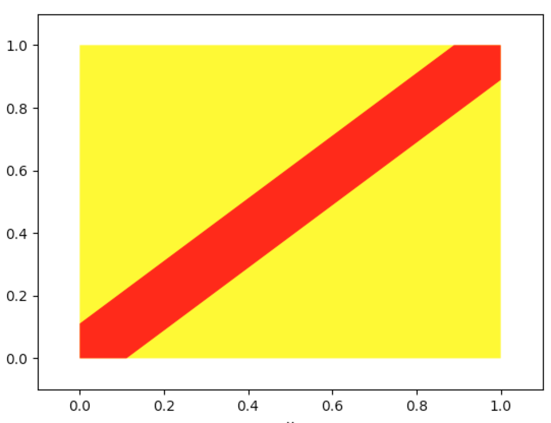
We can graph the region of integration:
In [77]: import numpy as np

In [78]: import matplotlib.pyplot as plt

In [79]: def grp_reg_ineff(fn1,fn2,xlb,xub,ylb,yub,xlim_lft=None,xlim_rgt=None,ymin=None,ymax=None,integrate_color='gr
    ...: een',bounds_color='yellow'):
    ...:     x_rng=np.arange(xlb,xub,0.0001)
    ...:     x=np.array(x_rng)
    ...:     y1,y2=[],[]
    ...:     for i in x:
    ...:         y1.append(min(max(fn1(i),ylb),yub))
    ...:         y2.append(min(max(fn2(i),ylb),yub))
    ...:     fig, (ax1) = plt.subplots(1, 1, sharex=True)
    ...:     ax1.fill_between(x, ylb, yub, facecolor=bounds_color)
    ...:     ax1.fill_between(x, y1, y2, facecolor=integrate_color)
    ...:     ax1.set_xlabel('x')
    ...:     ax1.set_xlim(xlim_lft if xlim_lft is not None else xlb,xlim_rgt if xlim_rgt is not None else xub)
    ...:     plt.ylim(ymin if ymin is not None else ylb, ymax if ymax is not None else yub)
    ...:     plt.show()
    ...:

In [80]: grp_reg_ineff(lambda x:x-1/9,lambda x:x+1/9,0,1,0,1,-0.1,1.1,-0.1,1.1,integrate_color='red')
(6.15.a)
$$ 1=\iint_{x,y\in R}\pdf{x,y}dxdy=c\wts\iint_{x,y\in R}dxdy=c\wts A(R) $$
where $A(R)$ is the area of the region $R$. Hence $A(R)=\frac1c$.
(6.15.b)
The square centered at the origin with sides of length $2$ has area $4=2\wts2$. From part (a), we know that $\pdf{x,y}=\frac14$. We can factor this as
$$ \pdf{x,y}=\frac14=\frac12\frac12=\pdfa{x}{X}\wts\pdfa{y}{Y} $$
And it was given that $x,y\in(-1,1)$.
(6.15.c)
$$ \pr{X^2+Y^2\leq1}=\iint_{x^2+y^2\leq1}\pdf{x,y}dxdy=\frac14\iint_{x^2+y^2\leq1}dxdy=\frac14\pi1^2=\frac\pi4 $$
(6.16.a)
$$ A=\cup_iA_i $$
Suppose $x\in A$. Then all the points are contained in some semicircle. So $x\in A_j\subset\cup_iA_i$ for some $j$.
Conversely, suppose $x\in\cup_iA_i$. Then $x\in A_j$ for some $j$. Then all the points are contained in the semicircle starting at the point $P_j$. So $x\in A$.
(6.16.b)
Yes they are disjoint. Proof by contradiction: Suppose that $A_j$ and $A_k$ both occur, $j\neq k$. Then the semicircles beginning at the points $P_j$ and $P_k$ each contain all the points $\set{P_i:1\leq i\leq n}$.
In particular, the semicircle beginning at $P_j$ contains $P_k$ and the semicircle beginning at $P_k$ contains $P_j$. That is, let $D_{jk}$ denote the distance on the circle from $P_j$ to $P_k$ and let $D_{kj}$ denote the distance on the circle from $P_k$ to $P_j$. Then $D_{jk}<\pi r$ and $D_{kj}<\pi r$ where $r$ is the radius of the circle. So $D_{jk}+D_{kj}<2\pi r$.
But $D_{jk}+D_{kj}=2\pi r$ since this is the distance of the path from $P_j$ to $P_k$ to $P_j$. That is, $D_{jk}+D_{kj}$ is the circumference of the circle.
(6.16.c)
First consider $A_1$. The location of $P_2$ is (presumably) uniformly distributed on $(0,2\pi r)$. So there is a probability of $\frac12$ that $P_2$ is contained in any given semicircle and, in particular, the semicircle starting at $P_1$. And there is a probability of $\frac12$ that $P_3$ is contained in the semicircle starting at $P_1$. And so on. Hence
$$ \pr{A_1}=\fracpB12^{n-1} $$
We can similarly show that for all $1\leq i\leq n$, we have
$$ \pr{A_i}=\fracpB12^{n-1} $$
Hence
$$ \pr{A}=\pr{\cup_i^nA_i}=\sum_i^n\pr{A_i}=\sum_i^n\fracpB12^{n-1}=n\fracpB12^{n-1} $$
(6.17)
Assume that the $3$ points have the same distribution. Then, by symmetry, all orderings of $X_1,X_2,X_3$ are equally likely. That is, the problem is the same if we relabel any of the three variables.
Of the $3!$ possible orderings, $2$ of them have $X_2$ in the middle. Hence there is a probability of $\frac2{3!}=\frac13$ of $X_2$ being between the other two points.
(6.18)
The marginal densities are
$$ \pdfa{x}{X}=\frac1{\frac{L}2-0}=\frac2L=\frac1{L-\frac{L}2}=\pdfa{y}{Y} $$
From the independence assumption, the joint density is
$$ \pdf{x,y}=\pdfa{x}{X}\wts\pdfa{y}{Y}=\frac4{L^2} $$
The WRONG solution is
$$ \prB{Y-X>\frac{L}3}=\prB{Y>X+\frac{L}3}=\int_{0}^{\frac{L}2}\int_{x+\frac{L}3}^{L}\pdf{x,y}dydx=\frac4{L^2}\int_{0}^{\frac{L}2}\int_{x+\frac{L}3}^{L}dydx $$
This is wrong because when $0\leq x\leq\frac{L}6$, then
$$ 0+\frac{L}3=\frac{L}3\leq\text{lower limit of the integral of }y\leq\frac{L}2=\frac{L}6+\frac{L}3 $$
For example, when $x=\frac{L}9$, then the inside integral should be
$$ \int_{\frac{L}9+\frac{L}3}^{L}\pdf{x,y}dy=\int_{\frac{4L}9}^{L}\pdf{x,y}dy=\int_{\frac{4L}9}^{\frac{L}2}0dy+\frac4{L^2}\int_{\frac{L}2}^{L}dy $$
To prevent $y$ from being integrated below $\frac{L}2$, we break up the integral:
$$ \prB{Y-X>\frac{L}3}=\prB{Y>X+\frac{L}3} $$
$$ =\int_{0}^{\frac{L}6}\int_{\frac{L}2}^{L}\pdf{x,y}dydx+\int_{\frac{L}6}^{\frac{L}2}\int_{x+\frac{L}3}^{L}\pdf{x,y}dydx $$
$$ =\frac4{L^2}\int_{0}^{\frac{L}6}\int_{\frac{L}2}^{L}dydx+\frac4{L^2}\int_{\frac{L}6}^{\frac{L}2}\int_{x+\frac{L}3}^{L}dydx $$
$$ =\frac4{L^2}\Cbr{\int_{0}^{\frac{L}6}\Prn{L-\frac{L}2}dx+\int_{\frac{L}6}^{\frac{L}2}\Sbr{L-\Prn{x+\frac{L}3}}dx} $$
$$ =\frac4{L^2}\Cbr{\frac{L}2\int_{0}^{\frac{L}6}dx+\int_{\frac{L}6}^{\frac{L}2}\Sbr{\frac{2L}3-x}dx} $$
$$ =\frac4{L^2}\Cbr{\frac{L}2\frac{L}6+\frac{2L}3\int_{\frac{L}6}^{\frac{L}2}dx-\int_{\frac{L}6}^{\frac{L}2}xdx} $$
$$ =\frac4{L^2}\Cbr{\frac{L^2}{12}+\frac{2L}3\Prn{\frac{L}2-\frac{L}6}-\frac12\Prn{x^2\eval{\frac{L}6}{\frac{L}2}}} $$
$$ =\frac4{L^2}\Cbr{\frac{L^2}{12}+\frac{2L}3\frac{L}3-\frac12\Prn{\frac{L^2}4-\frac{L^2}{36}}} $$
$$ =4\Cbr{\frac1{12}+\frac29-\frac12\Prn{\frac14-\frac1{36}}} $$
$$ =4\Cbr{\frac3{36}+\frac8{36}-\frac12\Prn{\frac9{36}-\frac1{36}}} $$
$$ =4\Cbr{\frac{11}{36}-\frac12\frac8{36}}=4\Cbr{\frac{11}{36}-\frac4{36}}=4\wts\frac7{36}=\frac79 $$
In [77]: import numpy as np
In [78]: import matplotlib.pyplot as plt
In [79]: def grp_reg_ineff(fn1,fn2,xlb,xub,ylb,yub,xlim_lft=None,xlim_rgt=None,ymin=None,ymax=None,integrate_color='gr ...: een',bounds_color='yellow'):
...: x_rng=np.arange(xlb,xub,0.0001)
...: x=np.array(x_rng)
...: y1,y2=[],[]
...: for i in x:
...: y1.append(min(max(fn1(i),ylb),yub))
...: y2.append(min(max(fn2(i),ylb),yub))
...: fig, (ax1) = plt.subplots(1, 1, sharex=True)
...: ax1.fill_between(x, ylb, yub, facecolor=bounds_color)
...: ax1.fill_between(x, y1, y2, facecolor=integrate_color)
...: ax1.set_xlabel('x')
...: ax1.set_xlim(xlim_lft if xlim_lft is not None else xlb,xlim_rgt if xlim_rgt is not None else xub)
...: plt.ylim(ymin if ymin is not None else ylb, ymax if ymax is not None else yub)
...: plt.show()
...:
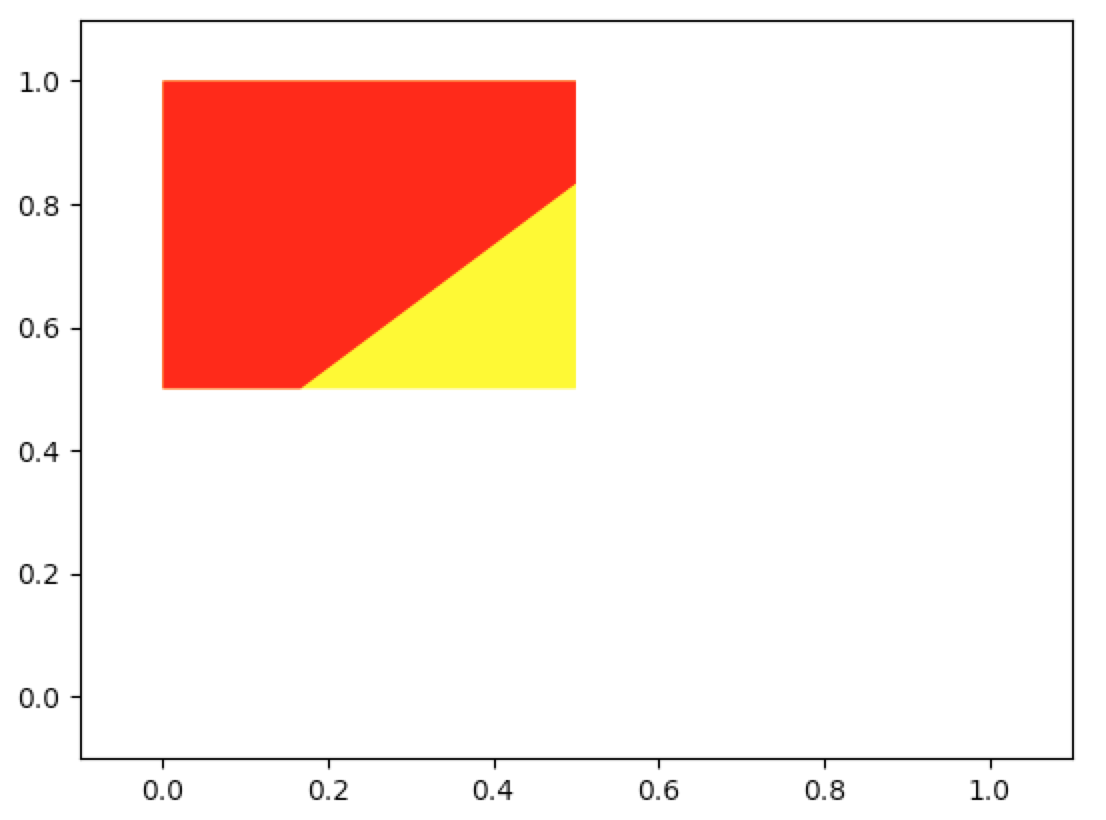
In [81]: grp_reg_ineff(lambda x:1,lambda x:x+1/3,0,1/2,1/2,1,-0.1,1.1,-0.1,1.1,integrate_color='red')
(6.19)
This is a really interesting example.
We verify that the function integrates to $1$ and is thus a joint density:
$$ \int_{0}^{1}\int_{y}^{1}\frac{dx}xdy=\int_0^1\Cbr{\ln{x}\eval{y}1}dy=\int_0^1\Cbr{0-\ln{y}}dy=-\int_0^1\ln{y}dy \tag{6.19.1} $$
$$ u=\ln{y}\dq du=\frac{dy}y\dq dv=1dy\dq v=y $$
$$ \int\ln{y}dy=\int udv=uv-\int vdu=y\ln{y}-\int y\frac{dy}y $$
$$ =y\ln{y}-\int dy=y\ln{y}-y \tag{6.19.2} $$
So $6.19.1$ becomes
$$ -\int_0^1\ln{y}dy=-\Prn{\Cbr{y\ln{y}-y}\eval01} $$
$$ =-\Prn{1\ln{1}-1-\prn{0\ln{0}-0}} $$
$$ =-\Prn{-1-\prn{-0}}=-\prn{-1}=1 $$
In [131]: I2(lambda x,y:1/x,0,1,lambda y:y,lambda y:1)
Out[131]: 1.0000000000000007
Are $X$ and $Y$ independent? Let’s recall Proposition 2.1:
The continuous random variables $X$ and $Y$ are independent if and only if their joint density can be factored into two terms, one depending only on $x$ and the other depending only on $y$. That is, $X,Y$ are independent IFF the joint density can be expressed as
$$ \pdfa{x,y}{X,Y}=h(x)\wts g(y) $$
Subtlety: the proposition makes no reference to the marginal densities of $X$ and $Y$. That is, $h(x)$ may or may not be the marginal density of $X$ and $g(y)$ may or may not be the marginal density of $y$.
Using this proposition, it would seem that $X$ and $Y$ are independent:
$$ \pdf{x,y}=\frac1x\wts1=h(x)\wts g(y) $$
where $h(x)=\frac1x$ and $g(y)=1$. But note that boundary: $0<y<x<1$. Hence dependency.
(6.19.a)
For $y\in(0,1)$, the marginal density of $Y$ is
$$ \pdfa{y}{Y}=\int_y^1\pdf{x,y}dx=\int_y^1\frac{dx}x=\ln{x}\eval{y}1=0-\ln{y}=-\ln{y} $$
Notice that the marginal density is not equal to the function $g$ from the first part:
$$ \pdfa{y}{Y}=-\ln{y}\neq1=g(y) $$
(6.19.b)
For $x\in(0,1)$, the marginal density of $X$ is
$$ \pdfa{x}{X}=\int_0^x\pdf{x,y}dy=\frac1x\int_0^xdy=\frac1xx=1 $$
Notice that the marginal density is not equal to the function $h$ from the first part:
$$ \pdfa{x}{X}=1\neq\frac1x=h(x) $$
Questions arise: (1) Is $\pdfa{x}{X}\wts\pdfa{y}{Y}=-\ln{y}$ a joint density? (2) It doesn’t integrate to $1$ (see below) so I guess not? (3) Are $X$ and $Y$ not independent?
Subsequent note: recall the boundary: $0<y<x<1$. Hence dependency.
$$ \int_0^1\int_y^1-\ln{y}dxdy=-\int_0^1\ln{y}\int_y^1dxdy=-\int_0^1\ln{y}(1-y)dy $$
$$ =\int_0^1y\ln{y}dy-\int_0^1\ln{y}dy $$
$$ =\Prn{\frac{y^2}2\ln{y}-\frac{y^2}4}\eval01-\Cbr{\prn{y\ln{y}-y}\eval01} \tag{By 6.19.d.2 and 6.19.2} $$
$$ =\frac{1^2}2\ln{1}-\frac{1^2}4-\Cbr{1\ln{1}-1}=-\frac14+1=\frac34 $$
In [118]: I2(lambda x,y:-np.log(y),0,1,lambda y:y,lambda y:1)
Out[118]: 0.7500000000000002
(6.19.c)
$$ \evw{X}=\int_0^1x\wts1dx=\frac12 $$
(6.19.d)
$$ \evw{Y}=-\int_0^1y\ln{y} dy \tag{6.19.d.1} $$
$$ u=\ln{y}\dq du=\frac{dy}y\dq dv=ydy\dq v=\frac{y^2}2 $$
$$ \int y\ln{y}dy=uv-\int vdu=\frac{y^2}2\ln{y}-\int\frac{y^2}2\frac{dy}y $$
$$ =\frac{y^2}2\ln{y}-\frac12\int ydy=\frac{y^2}2\ln{y}-\frac12\frac{y^2}2=\frac{y^2}2\ln{y}-\frac{y^2}4 \tag{6.19.d.2} $$
So 6.19.d.1 becomes
$$ \evw{Y}=-\int_0^1y\ln{y} dy=-\Prn{\frac{1^2}2\ln{1}-\frac{1^2}4}=\frac14 $$
(6.20.a)
By Proposition 2.1, $X$ and $Y$ are independent if and only if their joint probability density function can be factored into two terms, one depending only on $x$ and the other depending only on $y$.
$$ \pdf{x,y}=x\e{-(x+y)}=x\e{-x}\e{-y}=\pdfa{x}{X}\wts\pdfa{y}{Y} $$
where $\pdfa{x}{X}=x\e{-x}$ and $\pdfa{y}{Y}=\e{-y}$. And we can check that each of these is a density:
$$ \int_0^\infty\pdfa{x}{X}dx=\int_0^\infty x\e{-x}dx=\GammaF{2}=(2-1)!=1 \tag{6.20.a.1} $$
Or we can integrate by parts:
$$ u=x\dq du=dx\dq dv=\e{-x}dx\dq v=-\e{-x} $$
$$ \int x\e{-x}dx=uv-\int vdu=-x\e{-x}+\int\e{-x}dx=-x\e{-x}-\e{-x}=-\e{-x}(x+1) \tag{6.20.a.2} $$
So 6.20.a.1 becomes
$$ \int_0^\infty x\e{-x}dx=\prn{-\e{-x}(x+1)}\eval0\infty=\prn{\e{-x}(x+1)}\eval\infty0 $$
$$ =\e{-0}(0+1)-\prn{\e{-\infty}(\infty+1)}=1-\prn{0\wts\infty}=1 $$
And the marginal density of $y$ also integrates to $1$:
$$ \int_0^\infty\pdfa{y}{Y}dy=\int_0^\infty\e{-y}dy=\GammaF{1}=(1-1)!=0!=1 $$
or
$$ \int_0^\infty\pdfa{y}{Y}dy=\int_0^\infty\e{-y}dy=-\e{-y}\eval0\infty=\e{-y}\eval\infty0=1-0=1 $$
Note that we can derive the marginal densities this way:
$$ \pdfa{x}{X}=\int_{0}^{\infty}\pdf{x,y}dy=\int_{0}^{\infty}x\e{-(x+y)}dy=x\e{-x}\int_0^\infty\e{-y}dy=x\e{-x} $$
$$ \pdfa{y}{Y}=\int_{0}^{\infty}\pdf{x,y}dx=\int_{0}^{\infty}x\e{-(x+y)}dx=\e{-y}\int_0^\infty x\e{-x}dx=\e{-y} $$
(6.20.b)
Marginal densities:
$$ \pdfa{x}{X}=\int_{x}^{1}\pdf{x,y}dy=2\int_{x}^{1}dy=2(1-x) $$
$$ \pdfa{y}{Y}=\int_{0}^{1}\pdf{x,y}dx=2\int_{0}^{1}dx=2y $$
Hence $X$ and $Y$ are not independent since their joint density is not the product of the two marginal densities:
$$ \pdf{x,y}=2\neq4y(1-x)=\pdfa{x}{X}\wts\pdfa{y}{Y} $$
(6.21.a)
$$ \iint_{\substack{0\leq x\leq1\\0\leq y\leq1\\0\leq x+y\leq1}}\pdf{x,y}dydx=\iint_{\substack{0\leq x\leq1\\0\leq y\leq1\\-x\leq y\leq1-x}}\pdf{x,y}dydx=\iint_{\substack{0\leq x\leq1\\0\leq y\leq1-x}}\pdf{x,y}dydx $$
The last equation follows because, for all $x\in[0,1]$, we have $-x\leq0$ and $1-x\leq1$. Continuing:
$$ =\int_{0}^{1}\int_{0}^{1-x}\pdf{x,y}dydx=\int_{0}^{1}\int_{0}^{1-x}24xydydx $$
$$ =24\int_{0}^{1}x\int_{0}^{1-x}ydydx $$
$$ =24\wts\frac12\int_{0}^{1}x(1-x)^2dx $$
$$ =12\int_{0}^{1}x(1-2x+x^2)dx $$
$$ =12\int_{0}^{1}(x-2x^2+x^3)dx $$
$$ =12\Cbr{\Prn{\frac{x^2}2-2\frac{x^3}3+\frac{x^4}4}\eval01} $$
$$ =12\Cbr{\frac{1^2}2-2\frac{1^3}3+\frac{1^4}4} $$
$$ =12\Cbr{\frac12-\frac23+\frac14}=12\Cbr{\frac34-\frac23}=12\Cbr{\frac9{12}-\frac8{12}}=12\wts\frac1{12}=1 $$
(6.21.b)
For $x\in(0,1)$:
$$ \pdfa{x}{X}=\int_0^{1-x}\pdf{x,y}dy=\int_0^{1-x}24xydy=24x\int_0^{1-x}ydy $$
$$ =24x\frac12\Prn{y^2\eval0{1-x}}=12x(1-x)^2 $$
So the expected value of $X$ is
$$ \evw{X}=\int_0^1x\pdfa{x}{X}dx=\int_0^112x^2(1-x)^2dx $$
In [132]: I(lambda x:12*pw(x,2)*pw(1-x,2),0,1)
Out[132]: 0.3999999999999999
(6.21.c)
For $y\in(0,1)$:
$$ \pdfa{y}{Y}=\int_0^{1-y}\pdf{x,y}dx=\int_0^{1-y}24xydx=24y\int_0^{1-y}xdx $$
$$ =24y\frac12\Prn{x^2\eval0{1-y}}=12y(1-y)^2 $$
So the expected value of $Y$ is
$$ \evw{Y}=\int_0^1y\pdfa{y}{Y}dy=\int_0^112y^2(1-y)^2dy $$
(6.22.a)
For $x\in(0,1)$:
$$ \pdfa{x}{X}=\int_0^{1}\pdf{x,y}dy=\int_0^{1}(x+y)dy=x\int_0^{1}dy+\int_0^{1}ydy=x+\frac12 $$
For $y\in(0,1)$:
$$ \pdfa{y}{Y}=\int_0^{1}\pdf{x,y}dx=\int_0^{1}(x+y)dx=y\int_0^{1}dx+\int_0^{1}xdx=y+\frac12 $$
So $X$ and $Y$ are not independent since the product of their marginals is not equal to joint density.
(6.22.c)
$$ \pr{X+Y<1}=\pr{X<1-Y}=\int_0^1\int_0^{1-y}(x+y)dxdy $$
$$ =\int_0^1\Cbr{\int_0^{1-y}xdx+y\int_0^{1-y}dx}dy $$
$$ =\int_0^1\Cbr{\frac12\Sbr{x^2\eval0{1-y}}+y(1-y)}dy $$
$$ =\int_0^1\Cbr{\frac12(1-y)^2+y-y^2}dy $$
$$ =\int_0^1\Cbr{\frac12(1-2y+y^2)+y-y^2}dy $$
$$ =\int_0^1\Cbr{\frac12-y+\frac12y^2+y-y^2}dy $$
$$ =\int_0^1\Cbr{\frac12-\frac12y^2}dy $$
$$ =\frac12\int_0^1\cbr{1-y^2}dy $$
$$ =\frac12\Cbr{\int_0^1dy-\int_0^1y^2dy} $$
$$ =\frac12\Cbr{1-\frac13\Sbr{y^3\eval01}}=\frac12\Cbr{1-\frac13}=\frac12\frac23=\frac13 $$
(6.23.a)
For $x\in(0,1)$:
$$ \pdfa{x}{X}=\int_0^112xy(1-x)dy=12x\Cbr{\int_0^1ydy-\int_0^1yxdy} $$
$$ =12x\Cbr{\int_0^1ydy-x\int_0^1ydy} $$
$$ =12x\Cbr{\int_0^1ydy(1-x)} $$
$$ =12x(1-x)\int_0^1ydy $$
$$ =12x(1-x)\frac12\Sbr{y^2\eval01}=6x(1-x) $$
For $y\in(0,1)$:
$$ \pdfa{y}{Y}=\int_0^112xy(1-x)dx=12y\int_0^1x(1-x)dx $$
$$ =12y\Cbr{\int_0^1xdx-\int_0^1x^2dx} $$
$$ =12y\Cbr{\frac12\Sbr{x^2\eval01}-\frac13\Sbr{x^3\eval01}}=12y\Cbr{\frac12-\frac13}=12y\Cbr{\frac36-\frac26}=12y\frac16=2y $$
Hence $X$ and $Y$ are independent: for $x\in(0,1)$ and $y\in(0,1)$ we have
$$ \pdfa{x}{X}\wts\pdfa{y}{Y}=6x(1-x)2y=12xy(1-x)=\pdf{x,y} $$
(6.23.b)
$$ \evw{X}=\int_0^1x\pdfa{x}{X}dx=6\int_0^1x^2(1-x)dx $$
$$ =6\Cbr{\int_0^1x^2dx-\int_0^1x^3dx} $$
$$ =6\Cbr{\frac13\Sbr{x^3\eval01}-\frac14\Sbr{x^4\eval01}}=6\Cbr{\frac13-\frac14}=6\Cbr{\frac4{12}-\frac3{12}}=\frac12 $$
(6.23.c)
$$ \evw{Y}=\int_0^1y\pdfa{y}{Y}dy=2\int_0^1y^2dy=\frac23\Sbr{y^3\eval01}=\frac23 $$
(6.23.d)
$$ \evw{X^2}=\int_0^1x^2\pdfa{x}{X}dx=6\int_0^1x^3(1-x)dx $$
$$ =6\Cbr{\int_0^1x^3dx-\int_0^1x^4dx} $$
$$ =6\Cbr{\frac14\Sbr{x^4\eval01}-\frac15\Sbr{x^5\eval01}}=6\Cbr{\frac14-\frac15}=6\Cbr{\frac5{20}-\frac4{20}}=\frac6{20}=\frac3{10} $$
So the variance is
$$ \varw{X}=\evw{X^2}-\prn{\evw{X}}^2=\frac3{10}-\fracpB12^2=\frac{12}{40}-\frac{10}{40}=\frac2{40}=\frac1{20} $$
(6.23.e)
$$ \evw{Y^2}=\int_0^1y^2\pdfa{y}{Y}dy=2\int_0^1y^3dy=\frac24\Sbr{y^4\eval01}=\frac12 $$
So the variance is
$$ \varw{Y}=\evw{Y^2}-\prn{\evw{Y}}^2=\frac12-\fracpB23^2=\frac12-\frac49=\frac9{18}-\frac8{18}=\frac1{18} $$
(6.24.a)
Some examples:
$$ \pr{N=1}=1-p_0\dq\pr{N=2}=p_0(1-p_0)\dq\pr{N=3}=p_0^2(1-p_0) $$
Hence $N$ is a geometric random variable with parameter $1-p_0$:
$$ \pr{N=n}=p_0^{n-1}(1-p_0) $$
(6.24.b)
We can solve this in two ways.
First solution: the result of $X$ must be an integer from $1$ through $k$. And it should be that $\pr{X=j}=cp_j$ for some $c>0$. That is, for each $j=1,…,k$, the probability that $X=j$ should be proportional to $p_j$. But the sum of the probabilities over all possible values of $X$ should be $1$. Hence
$$ 1=\sum_{j=1}^k\pr{X=j}=\sum_{j=1}^kcp_j=c\sum_{j=1}^kp_j=c\Prn{\sum_{j=0}^kp_j-p_0}=c(1-p_0) $$
Hence $c=\frac1{1-p_0}$ and $\pr{X=j}=\frac{p_j}{1-p_0}$.
Alternative solution: The condition on $X$ is that it doesn’t equal $0$ on some trial, call it trial $n$. Let $Y$ denote the unconditional outcome of trial $n$. So the possible values of $Y$ are $0,1,…,k$. Then for $j=1,…,k$, we have
$$ \set{Y=j}\subset\set{Y\neq0}\implies\set{Y=j}\cap\set{Y\neq0}=\set{Y=j} $$
and
$$ \pr{X=j}=\cp{Y=j}{Y\neq0}=\frac{\pr{Y=j,Y\neq0}}{\pr{Y\neq0}}=\frac{\pr{Y=j}}{\pr{Y\neq0}}=\frac{p_j}{1-p_0} $$
(6.24.c)
We have
$$ \pr{N=n,X=j}=\pr{N=n}\cp{X=j}{N=n} $$
From parts (a) and (b), we have
$$ \pr{N=n}=p_0^{n-1}(1-p_0)\dq\pr{X=j}=\frac{p_j}{1-p_0} $$
So we see that the value of $X$ doesn’t depend on the stopping time $N=n$. That is, $X$ and $N$ are independent. Hence
$$ \pr{N=n,X=j}=\pr{N=n}\cp{X=j}{N=n}=\pr{N=n}\pr{X=j} $$
$$ =p_0^{n-1}(1-p_0)\frac{p_j}{1-p_0}=p_0^{n-1}p_j $$
(6.24.d)
We wish to understand intuitively why the value of $X$ is irrelevant to determining when $N$ occurs. The reason is that the trials are independent and identically distributed (IID).
$X$ is the outcome of the first trial whose outcome is not $0$. From IID, for any distinct values $i,j$ with $1\leq i,j\leq k$, whether $X=i$ or $X=j$ is irrelevant to determining the observed value of $N$. So, intuitively, $N$ is independent of $X$ because the value of $X$ is irrelevant to determining when $N$ occurs.
If the trials are not independent or not identically distributed, then $N$ can be dependent on $X$. Suppose that the possible outcomes are $0,1,2$. Also suppose that trials with an even number have the probabilities $p_0=\frac12$, $p_1=0$, and $p_2=\frac12$ and that trials with an odd number have the probabilities $p_0=\frac12$, $p_1=\frac12$, and $p_2=0$.
Then the trials are not identically distributed. Moreover, if $X=1$, then it is certain that $N$ is an odd number and, if $X=2$, then it is certain that $N$ is an even number.
(6.24.e)
Note that the trials are independent and identically distributed. Hence, intuitively, $X$ is independent of $N$ because the stopping time in no way effects the outcome of the first trial whose outcome is not zero. That is, for any distinct integers $n\neq m$, whether $N=n$ or $N=m$ is irrelevant to determining the observed value of $X$.
(6.25)
Apparently we are meant to infer that the unit of time is hours. That is, for a given person, their arrival time is uniformly distributed over $(0,10^6)$ hours. Hence the probability that a person arrives during the $t^{th}$ hour is
$$ p\equiv\frac1{10^6}\int_t^{t+1}dx=\frac1{10^6}(t+1-t)=\frac1{10^6} $$
Note that
- $n=10^6$ (the number of people) is large
- $p=\frac1{10^6}$ is small
- the arrival times are independent
Hence we can compute the number of people that arrive in the first hour as a Binomial random variable or we can approximate this is a Poisson random variable.
$$ \pmfa{i}{X}=\binom{10^6}ip^i(1-p)^{10^6-i} $$
And the Poisson approximation with $\lambda=np=10^6\wts\frac1{10^6}=1$:
$$ \pmfa{i}{X}=\e{-\lambda}\frac{\lambda^i}{i!}=\e{-1}\frac{1^i}{i!}=\frac{\e{-1}}{i!} $$
In [173]: w_p6_25=lambda n=pw(10,6),p=1/pw(10,6),i=pw(10,5)*5:(winom(n,i)*pw(p,i)*pw(1-p,n-i),np.exp(-n*p)/wf(i))

In [174]: w_p6_25(i=1),w_p6_25(i=2),w_p6_25(i=3),w_p6_25(i=4)
Out[174]:
((0.367879625100692, 0.36787944117144233),
 (0.183939812550346, 0.18393972058572117),
 (0.0613132095367831, 0.061313240195240391),
 (0.0153282717275603, 0.015328310048810098))
(6.26.a)
For $a,b,c\in(0,1)$, from the independence assumption, we can compute the joint density
$$ \pdfa{a,b,c}{A,B,C}=\pdfa{a}{A}\wts\pdfa{b}{B}\wts\pdfa{c}{C}=1\wts1\wts1=1 $$
Hence the joint random variable $A,B,C$ is uniformly distributed over $(0,1)^3$ and for $a_0,b_0,c_0\in(0,1)$ we have
$$ \cdfa{a_0,b_0,c_0}{A,B,C}=\int_0^{c_0}\int_0^{b_0}\int_0^{a_0}\pdfa{a,b,c}{A,B,C}dadbdc $$
$$ =\int_0^{c_0}\int_0^{b_0}\int_0^{a_0}dadbdc $$
$$ =\int_0^{c_0}\int_0^{b_0}(a_0-0)dbdc $$
$$ =a_0\int_0^{c_0}\int_0^{b_0}dbdc $$
$$ =a_0\int_0^{c_0}(b_0-0)dc=a_0b_0\int_0^{c_0}dc=a_0b_0c_0 $$
Or we can compute the joint distribution from the definition: for $a,b,c\in(0,1)$, we have
$$ \cdfa{a,b,c}{A,B,C}=\pr{A\leq a,B\leq b,C\leq c}=\pr{A\leq a}\pr{B\leq b}\pr{C\leq c}=abc $$
where the second equation follows from independence and the last equation follows from
$$ \pr{A\leq a}=\int_0^a\pdfa{x}{A}dx=a $$
(6.26.b)
Recall the quadratic formula:
$$ A^2x+Bx+C=0\implies x=\frac{-B\pm\sqrt{B^2-4AC}}{2A} $$
So $x$ will be real exactly when $B^2-4AC\geq0$. So we wish to compute this probability. To do so, we first compute the density of the product $A\wt C$. To do that, we first compute its distribution. Note that for $x,a,c\in(0,1)$, we have
$$ ac\leq x\iff c\leq\frac{x}{a} $$
And the distribution is
$$ \cdfa{x}{A\wt C}=\pr{AC\leq x}=\iint_{\substack{c\leq\frac{x}a\\0\leq a\leq1\\0\leq c\leq1}}dcda $$
$$ =\int_0^x\int_0^1dcda+\int_x^1\int_0^{\frac{x}a}dcda \tag{6.26.b.1} $$
The limits of integration follow because
$$ \cases{a<x\implies\frac{x}a>1\geq c&\text{for all }c\in(0,1)\\a>x\implies\frac{x}a<1\implies c\leq\frac{x}a&\text{only for }c\leq\frac{x}a} $$
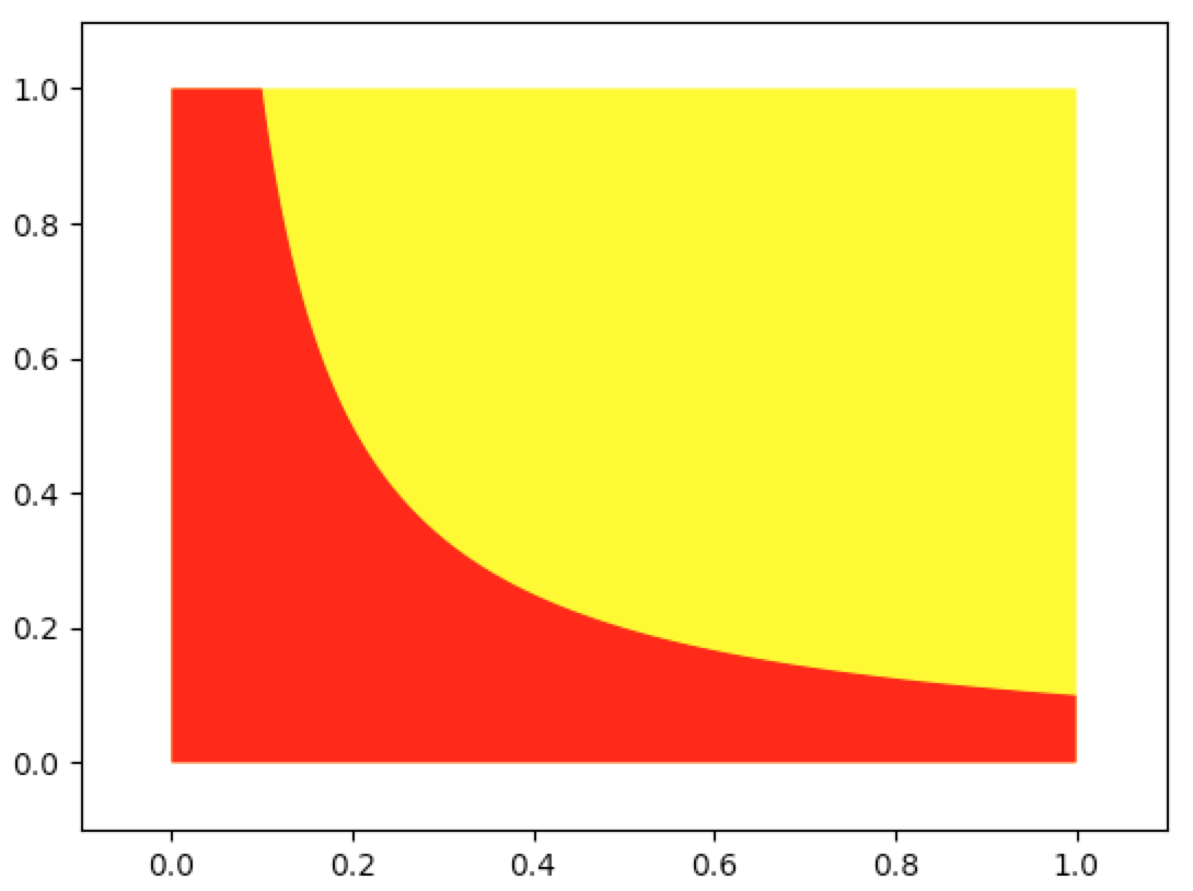
In [91]: grp_reg_ineff(lambda a:0,lambda a,x=1/10:x/a,0,1,0,1,-0.1,1.1,-0.1,1.1,integrate_color='red')
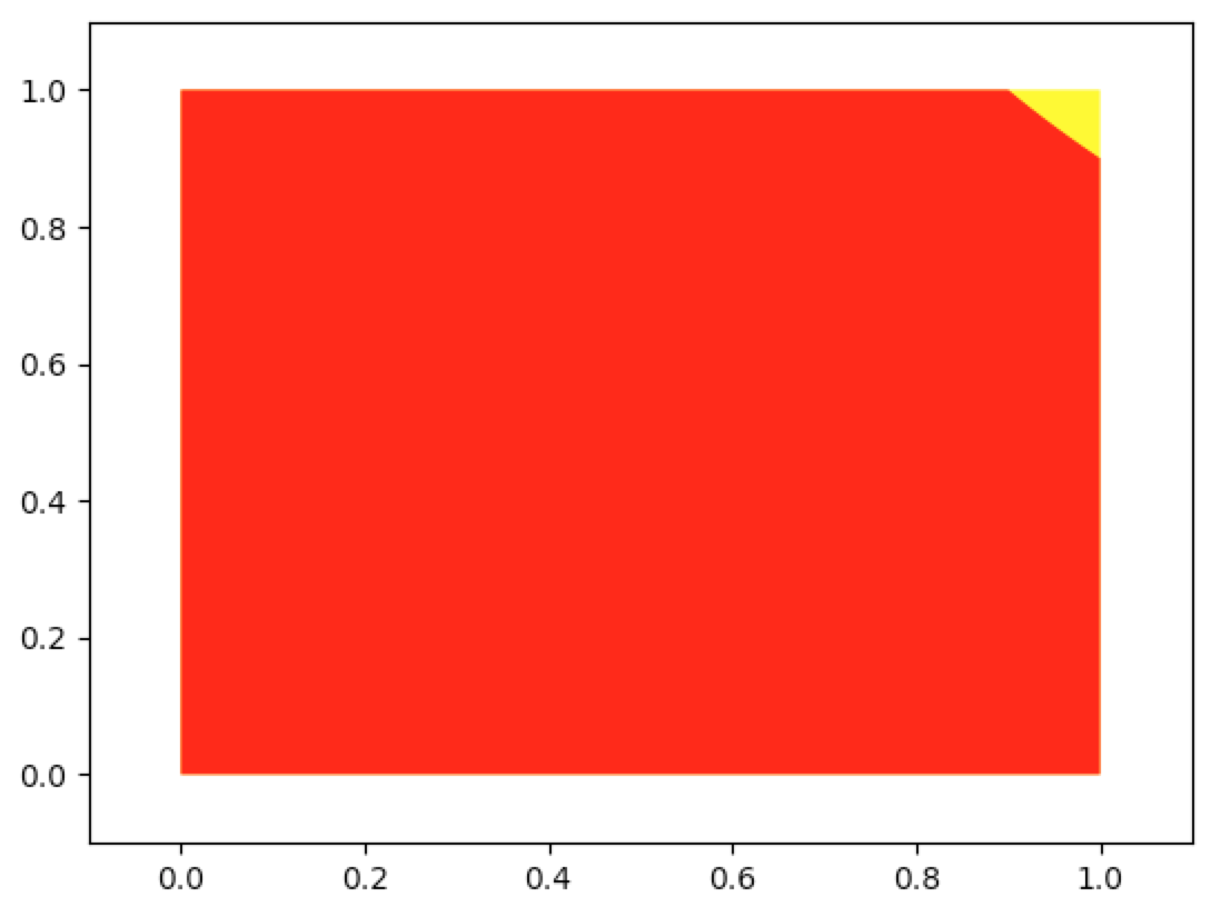
In [91]: grp_reg_ineff(lambda a:0,lambda a,x=9/10:x/a,0,1,0,1,-0.1,1.1,-0.1,1.1,integrate_color='red')
Then 6.26.b.1 becomes
$$ \cdfa{x}{A\wt C}=\int_0^x\int_0^1dcda+\int_x^1\int_0^{\frac{x}a}dcda=\int_0^xda+\int_x^1\frac{x}ada $$
$$ =x+x\int_x^1\frac{da}a=x+x\Prn{\ln{a}\eval{x}1}=x+x\prn{\ln1-\ln{x}}=x-x\ln{x} $$
Then the density of $A\wt C$ is
$$ \pdfa{x}{A\wt C}=\wderiv{F_{A\wt C}}{x}=1-\prn{1\wts\ln{x}+x\wts\frac1x}=1-\prn{\ln{x}+1}=-\ln{x} $$
Also note that the independence of $A$, $B$, and $C$ implies the independence of $A\wt C$ and $B$. Hence $\pdfa{x,b}{A\wt C,B}=\pdfa{x}{A\wt C}\pdfa{b}{B}$ and
$$ \pr{B^2-4AC\geq0}=\pr{B^2>4AC}=\prB{AC<\frac{B^2}4}=\int_0^1\int_{0}^{\frac{b^2}4}\pdfa{x}{A\wt C}\pdfa{b}{B}dxdb $$
$$ =-\int_0^1\int_{0}^{\frac{b^2}4}\ln{x}dxdb $$
$$ =-\int_0^1\Sbr{(x\ln{x}-x)\eval{0}{\frac{b^2}4}}db \tag{from 6.19.2} $$
$$ =-\int_0^1\Cbr{\frac{b^2}4\ln{\frac{b^2}4}-\frac{b^2}4}db $$
$$ =\int_0^1\Cbr{\frac{b^2}4-\frac{b^2}4\ln{\frac{b^2}4}}db \tag{6.26.b.2} $$
In [176]: I(lambda b:(1/4)*pw(b,2)-(1/4)*pw(b,2)*np.log((1/4)*pw(b,2)),0,1)
Out[176]: 0.25441341898203773
The solutions manual uses the identity
$$ \int x^2\ln{x}dx=\frac{x^3\ln{x}}3-\frac{x^3}9 $$
to compute the integral in 6.26.b.2. I’m not looking to become a professional integrater just yet so scipy.integrate is good for now. Plus I don’t really follow this math.
(6.27)
We compute the joint density. For $x_1,x_2>0$, from the independence assumption, we have
$$ \pdfa{x_1,x_2}{X_1,X_2}=\pdfa{x_1}{X_1}\wts\pdfa{x_2}{X_2}=\lambda_1\e{-\lambda_1x_1}\lambda_2\e{-\lambda_2x_2} $$
And the distribution of $Z=\frac{X_1}{X_2}$ is
$$ \cdfa{z}{Z}=\pr{Z<z}=\prB{\frac{X_1}{X_2}<z}=\pr{X_1<zX_2} $$
$$ =\iint_{\substack{0<x_1<zx_2\\x_2>0}}\pdfa{x_1,x_2}{X_1,X_2}dx_1dx_2 $$
$$ =\int_{0}^{\infty}\int_{0}^{zx_2}\pdfa{x_1,x_2}{X_1,X_2}dx_1dx_2 $$
$$ =\int_{0}^{\infty}\int_{0}^{zx_2}\lambda_1\e{-\lambda_1x_1}\lambda_2\e{-\lambda_2x_2}dx_1dx_2 $$
$$ =\int_{0}^{\infty}\lambda_2\e{-\lambda_2x_2}\int_{0}^{zx_2}\lambda_1\e{-\lambda_1x_1}dx_1dx_2 $$
$$ =\int_{0}^{\infty}\lambda_2\e{-\lambda_2x_2}\Sbr{-\e{-\lambda_1x_1}\eval0{zx_2}}dx_2 $$
$$ =\int_{0}^{\infty}\lambda_2\e{-\lambda_2x_2}\Sbr{\e{-\lambda_1x_1}\eval{zx_2}0}dx_2 $$
$$ =\int_{0}^{\infty}\lambda_2\e{-\lambda_2x_2}\prn{1-\e{-\lambda_1zx_2}}dx_2 $$
$$ =\int_{0}^{\infty}\Cbr{\lambda_2\e{-\lambda_2x_2}-\lambda_2\e{-\lambda_2x_2}\e{-\lambda_1zx_2}}dx_2 $$
$$ =\int_{0}^{\infty}\lambda_2\e{-\lambda_2x_2}dx_2-\int_{0}^{\infty}\lambda_2\e{-\lambda_2x_2}\e{-\lambda_1zx_2}dx_2 $$
$$ =-\e{-\lambda_2x_2}\eval0\infty-\lambda_2\int_{0}^{\infty}\e{-x_2(\lambda_2+\lambda_1z)}dx_2 $$
$$ =\e{-\lambda_2x_2}\eval\infty0-\lambda_2\Sbr{-\frac1{\lambda_2+\lambda_1z}\e{-x_2(\lambda_2+\lambda_1z)}\eval0\infty} $$
$$ =1-0+\frac{\lambda_2}{\lambda_2+\lambda_1z}\Sbr{\e{-x_2(\lambda_2+\lambda_1z)}\eval0\infty} $$
$$ =1+\frac{\lambda_2}{\lambda_2+\lambda_1z}(0-1) $$
$$ =\frac{\lambda_2+\lambda_1z}{\lambda_2+\lambda_1z}-\frac{\lambda_2}{\lambda_2+\lambda_1z}=\frac{\lambda_1z}{\lambda_2+\lambda_1z} $$
Also
$$ \pr{X_1<X_2}=\prB{\frac{X_1}{X_2}<1}=\pr{Z<1}=\cdfa{1}{Z}=\frac{\lambda_1\wts1}{\lambda_2+\lambda_1\wts1}=\frac{\lambda_1}{\lambda_2+\lambda_1} $$
(6.28.a)
Let $X$ denote the service time for AJ’s car and let $Y$ denote the service time for MJ’s car. Then
$$ \pr{X-t>Y}=\pr{X>Y+t}=\iint_{\substack{x>y+t\\x>0\\y>0}}\pdfa{x,y}{X,Y}dxdy $$
$$ =\int_{0}^{\infty}\int_{y+t}^{\infty}\pdfa{x,y}{X,Y}dxdy $$
$$ =\int_{0}^{\infty}\int_{y+t}^{\infty}\e{-x}\e{-y}dxdy $$
$$ =\int_{0}^{\infty}\e{-y}\int_{y+t}^{\infty}\e{-x}dxdy $$
$$ =\int_{0}^{\infty}\e{-y}\Prn{-\e{-x}\eval{y+t}{\infty}}dy $$
$$ =\int_{0}^{\infty}\e{-y}\Prn{\e{-x}\eval{\infty}{y+t}}dy $$
$$ =\int_{0}^{\infty}\e{-y}\e{-y-t}dy $$
$$ =\e{-t}\int_{0}^{\infty}\e{-2y}dy $$
$$ =\e{-t}\Prn{-\frac12\e{-2y}\eval0\infty}=\frac12\e{-t}\Prn{\e{-2y}\eval\infty0}=\frac{\e{-t}}2 $$
Fun aside: Recall that the exponential random variable is memoryless:
$$ \cp{X>s+t}{X>t}=\pr{X>s}\iff\pr{X>s+t}=\pr{X>s}\pr{X>t} $$
since
$$ \pr{X>s}=\cp{X>s+t}{X>t}=\frac{\pr{X>s+t,X>t}}{\pr{X>t}}=\frac{\pr{X>s+t}}{\pr{X>t}} $$
(6.28.b)
Recall from Example 3b on p.255 that the sum of two independent exponential random variables, each with parameter $\lambda$, is a gamma random variable with parameters $(2,\lambda)$. Then
$$ \pdfa{t}{X+Y}=\frac{\lambda\e{-\lambda t}(\lambda t)^{2-1}}{\GammaF{2}}=\lambda^2t\e{-\lambda t} $$
so that with $\lambda=1$, we have
$$ \pr{X+Y<2}=\int_0^2t\e{-t}dt $$
$$ u=t\dq du=dt\dq dv=\e{-t}dt\dq v=-\e{-t} $$
$$ \pr{X+Y<2}=uv-\int vdu=-t\e{-t}\eval02+\int_0^2\e{-t}dt $$
$$ =t\e{-t}\eval20-\e{-t}\eval02=(0-2\e{-2})-(\e{-2}-1)=1-3\e{-2} $$
(6.29.a)
Let $X_i$ denote sales for week $i\geq1$. If we assume that the $\set{X_i:i\geq1}$ are independent, then from Proposition 3.2 on p.256, $W\equiv X_1+X_2$ is normally distributed with parameters
$$ \mu=2200+2200\dq\sigma^2=230^2+230^2 $$
Hence
$$ \pr{X_1+X_2>5000}=\pr{W>5000}=1-\pr{W<5000} $$
$$ =1-\prB{Z-\frac{5000-4400}{\sqrt{2\wts230^2}}}=1-\snB{\frac{5000-4400}{\sqrt{2\wts230^2}}} $$
In [177]: from scipy.stats import norm

In [178]: phi=lambda x:norm(0,1).cdf(x)

In [179]: 1-phi((5000-4400)/np.sqrt(2*pw(230,2)))
Out[179]: 0.032545953007749873
(6.29.b)
For a given week $j$, the probability that sales exceed $2K$ is
$$ p\equiv\pr{X_j>2K}=1-\pr{X_j<2K}=1-\prB{Z<\frac{2K-2200}{230}}=1-\snB{\frac{2K-2200}{230}} $$
In [180]: p=1-phi((2000-2200)/230)

In [181]: p
Out[181]: 0.80773097350168832
Now we have a binomial random variable:
$$ \prt{sales exceed 2K in at least 2 of next 3 weeks}=\sum_{i=2}^3\binom3ip^i(1-p)^{3-i} $$
In [182]: sum([winom(3,i)*pw(p,i)*pw(1-p,3-i) for i in range(2,4)])
Out[182]: 0.903313228120415
(6.30.a)
Let $X$ and $Y$ denote Jack’s and Jill’s scores. Since $X$ and $Y$ are approximately normal and independent, we know from Proposition 3.2 on p.256, that $Y-X=Y+(-X)$ will be approximately normal with parameters
$$ \mu_{Y-X}=\mu_Y+(-\mu_X)=170-160=10\dq $$
and
$$ \sigma_{Y-X}^2=\sigma_Y^2+\sigma_{-X}^2=\sigma_Y^2+\sigma_{X}^2=20^2+15^2 $$
Hence
$$ \pr{X>Y}\approx\pr{X>Y+0.5}=\pr{Y+0.5<X}=\pr{Y-X<-0.5} $$
$$ \approx\prB{Z<\frac{-0.5-\mu_{Y-X}}{\sigma_{Y-X}}}=\snB{\frac{-10.5}{\sqrt{20^2+15^2}}} $$
where we have used the continuity correction in the first approximation. Generally, continuity correction is applied when approximating a binomial distribution with a normal distribution. Should continuity correction generally be applied to any discrete approximation by a normal distribution?
In [201]: phi(-10.5/np.sqrt(pw(20,2)+pw(15,2))) # with continuity correction
Out[201]: 0.33724272684824952

In [202]: phi(-10/np.sqrt(pw(20,2)+pw(15,2))) # without continuity correction
Out[202]: 0.34457825838967582
Here’s another discrete approximation that closely matches the above approximation with continuity correction:
$$ \pr{X>Y}=\sum_{y=0}^{300}\sum_{x=y+1}^{300}\pdfa{x,y}{X,Y}=\sum_{y=0}^{300}\Cbr{\pdfa{y}{Y}\sum_{x=y+1}^{300}\pdfa{x}{X}} $$
$$ =\sum_{y=0}^{300}\Cbr{\frac1{20\sqrt{2\pi}}\e{-\frac{(y-170)^2}{2\wts20^2}}\sum_{x=y+1}^{300}\frac1{15\sqrt{2\pi}}\e{-\frac{(x-160)^2}{2\wts15^2}}} $$
In [214]: normaldens=lambda x=0,mu=0,sig=1:(1/(sig*np.sqrt(2*np.pi)))*np.exp(-pw(x-mu,2)/(2*pw(sig,2)))

In [215]: sum([normaldens(y,mu=170,sig=20)*sum([normaldens(x,mu=160,sig=15) for x in range(y+1,301)]) for y in range(0
     ...: ,301)])
Out[215]: 0.33723249814551071
If we (incorrectly) take $X$ and $Y$ to be continuous, then
$$ \pr{X>Y}=\iint_{\substack{300\geq x>y\\300\geq x\geq 0\\300\geq y\geq0}}\pdfa{x,y}{X,Y}dxdy $$
$$ =\int_0^{300}\int_y^{300}\pdfa{x}{X}\pdfa{y}{Y}dxdy $$
$$ =\int_0^{300}\frac1{20\sqrt{2\pi}}\e{-\frac{(y-170)^2}{2\wts20^2}}\int_y^{300}\frac1{15\sqrt{2\pi}}\e{-\frac{(x-160)^2}{2\wts15^2}}dxdy $$
In [225]: normaldens=lambda x=0,mu=0,sig=1:(1/(sig*np.sqrt(2*np.pi)))*np.exp(-pw(x-mu,2)/(2*pw(sig,2)))

In [226]: I2(lambda x,y:normaldens(x,mu=160,sig=15)*normaldens(y,mu=170,sig=20),0,300,lambda y:y,lambda y:300)
Out[226]: 0.3445782583896758

In [227]: phi(-10/np.sqrt(pw(20,2)+pw(15,2)))
Out[227]: 0.34457825838967582

In [228]: I2(lambda x,y:normaldens(x,mu=160,sig=15)*normaldens(y,mu=170,sig=20),0,300,lambda y:y+1/2,lambda y:300)
Out[228]: 0.33724272684824963

In [229]: phi(-10.5/np.sqrt(pw(20,2)+pw(15,2)))
Out[229]: 0.33724272684824952
Notice that the first computed integral is identical to the normal approximation without continuity correction whereas the second computed integral is nearly identical to the normal approximation with continuity correction.
So do we use continuity correction or not? When we run a large number of experiments, it definitely appears that we should apply continuity correction:
In [346]: from random import uniform

In [347]: def normal_disc_pcdf(bnum=2,anum=2,mu=0,sig=1):
     ...:     cdf=[]
     ...:     for i in range(mu-bnum,mu+anum+1):
     ...:         p=normaldens(x=i,mu=mu,sig=sig)
     ...:         pp=0 if len(cdf)==0 else cdf[-1][2]
     ...:         cdf.append((i,p,p+pp))
     ...:     return cdf
     ...:

In [348]: def get_normal_int(lb=0,ub=300,mu=160,sig=15):
     ...:     data=normal_disc_pcdf(bnum=mu-lb,anum=ub-mu,mu=mu,sig=sig)
     ...:     u=uniform(0,1)
     ...:     val=0
     ...:     for dt in data:
     ...:         # also handle case where this is the last dt in data, in
     ...:         # which case, this if condition should be true
     ...:         if u<=dt[2]:
     ...:             val=dt[0]
     ...:             break
     ...:     return val
     ...:

In [349]: def w_6_30a(n=1000):
     ...:     cnt=0
     ...:     for i in range(int(n)):
     ...:         X=get_normal_int(lb=0,ub=300,mu=160,sig=15)
     ...:         Y=get_normal_int(lb=0,ub=300,mu=170,sig=20)
     ...:         if X>Y: cnt+=1
     ...:     return cnt/n
     ...:

In [350]: w_6_30a(n=7e+4)
Out[350]: 0.3362

In [351]: w_6_30a(n=7e+4)
Out[351]: 0.3379
(6.30.b)
$$ \pr{X+Y>350}\approx\pr{X+Y>350.5}=1-\pr{X+Y<350.5}=1-\snB{\frac{350.5-(160+170)}{\sqrt{20^2+15^2}}} $$
In [353]: 1-phi((350.5-330)/np.sqrt(pw(20,2)+pw(15,2)))
Out[353]: 0.20610805358581308

In [354]: def w_6_30b(n=1000):
     ...:     cnt=0
     ...:     for i in range(int(n)):
     ...:         X=get_normal_int(lb=0,ub=300,mu=160,sig=15)
     ...:         Y=get_normal_int(lb=0,ub=300,mu=170,sig=20)
     ...:         if X+Y>350: cnt+=1
     ...:     return cnt/n
     ...:

In [355]: w_6_30b()
Out[355]: 0.201

In [356]: w_6_30b(7e+4)
Out[356]: 0.20624285714285714
(6.31.a)
The probability that a given man from the sample of $n=200$ never eats breakfast is $p_m=0.252$. And the probability that a given woman from the sample of $n=200$ never eats breakfast is $p_w=0.236$.
Let $X$ and $Y$ denote, respectively, the number of males and females in the sample that never eat breakfast. Then $X$ and $Y$ are binomial random variables with respective parameters $(200,0.252)$ and $(200,0.236)$.
We know from section 4.6.1, p.139, that for a binomial random variable $W$ with parameters $(n,p)$ that $\evw{W}=np$ and $\varw{W}=np(1-p)$. Hence
$$ \evw{X}=np_m=200\wts0.252=50.4\dq\varw{X}=np_m(1-p_m)=37.6992 $$
$$ \evw{Y}=np_w=200\wts0.236=47.2\dq\varw{Y}=np_w(1-p_w)=36.0608 $$
In [369]: n,pm,pw=200,.252,.236

In [370]: evx,varx=n*pm,n*pm*(1-pm)

In [371]: evy,vary=n*pw,n*pw*(1-pw)

In [372]: evx,varx,evy,vary
Out[372]: (50.4, 37.6992, 47.199999999999996, 36.0608)
We can approximate each binomial random variable with a normal random variable. And we know from Proposition 3.2 on p.256 that the sum of these normal approximations is itself approximately normal with parameters
$$ \mu_{X+Y}=\mu_X+\mu_Y=\evw{X}+\evw{Y}=97.6\dq\sigma_{X+Y}^2=\sigma_X^2+\sigma_Y^2=73.76 $$
In [377]: muxpy=evx+evy

In [378]: varxpy=varx+vary

In [379]: muxpy,varxpy
Out[379]: (97.6, 73.75999999999999)
Hence
$$ \pr{X+Y\geq110}\approx\pr{X+Y>109.5}=1-\pr{X+Y<109.5}=1-\snB{\frac{109.5-\mu_{X+Y}}{\sigma_{X+Y}}} $$
In [380]: 1-phi((109.5-muxpy)/np.sqrt(varxpy))
Out[380]: 0.082935205512856047
(6.31.b)
Applying the same ideas as above, we have
$$ \mu_{X-Y}=\mu_{X+(-Y)}=\mu_X+(-\mu_Y)=\evw{X}+\prn{-\evw{Y}}=\evw{X}-\evw{Y}=3.2 $$
$$ \sigma_{X-Y}^2=\sigma_{X+(-Y)}^2=\sigma_X^2+\sigma_{-Y}^2=\sigma_X^2+\sigma_Y^2=\sigma_{X+Y}^2 $$
In [382]: muxmy=evx-evy

In [383]: varxmy=varxpy

In [384]: muxmy,varxmy
Out[384]: (3.200000000000003, 73.75999999999999)
Hence
$$ \pr{Y\geq X}=\pr{X\leq Y}=\pr{X-Y\leq0}\approx\pr{X-Y<0.5}\approx\snB{\frac{0.5-\mu_{X-Y}}{\sigma_{X-Y}}} $$
In [386]: phi((.5-muxmy)/np.sqrt(varxmy))
Out[386]: 0.37661666182537479
(6.32.a)
This is a follow-up problem from 4.51.
Let $X_i$ be the number of typos on page $i$ of this $10$ page article. Then the expected number of typos on page $i$ is
$$ \lambda=\evw{X_i}=0.2 $$
Assumptions:
- the number of characters on each page is large and roughly the same, say $n_i=700$
- the probability that each character is a typo is small: $p=\frac\lambda{n_i}\approx\frac{.2}{700}\approx.0003$
- typos are independent
Hence $X_i$ is binomial with parameters $n_i$ and $p$. And $X_i$ can be approximated as Poisson with parameter $\lambda$.
From example 3f on p.260, we know $X_i+X_j$ is binomial with parameters $n=2\wts700$ and $p=\frac\lambda{n_i}$. By induction, we know that $\sum_{i=1}^{10}X_i$ is binomial with parameters $n=10\wts700=7K$ and $p=\frac\lambda{n_i}$.
From example 3e on p.259, we know that $X_i+X_j$ is Poisson with parameter $2\lambda$. By induction, we know that $\sum_{i=1}^{10}X_i$ is Poisson with parameter $10\lambda$.
$$ \pmfaB{0}{\sum_{i=1}^{10}X_i}=\binom{7K}{0}p^0(1-p)^{7K-0} $$
$$ \pmfaB{0}{\sum_{i=1}^{10}X_i}\approx\frac{\e{-10\lambda}(10\lambda)^0}{0!}=\e{-2} $$
In [426]: n,p,lam=7000,.2/700,2

In [427]: n,p,lam
Out[427]: (7000, 0.00028571428571428574, 2)

In [428]: winom(n,0)*pw(p,0)*pw(1-p,n-0)
Out[428]: 0.135296614171489

In [429]: np.exp(-2)
Out[429]: 0.1353352832366127
(6.32.b)
$$ \prB{\sum_{i=1}^{10}X_i\geq2}=1-\Prn{\prB{\sum_{i=1}^{10}X_i=0}+\prB{\sum_{i=1}^{10}X_i=1}} $$
$$ \approx1-\Prn{\e{-2}+\frac{\e{-10\lambda}(10\lambda)^1}{1!}} $$
$$ =1-\prn{\e{-2}+2\e{-2}}=1-3\e{-2} $$
In [430]: brv=lambda n=10,i=0,p=1/2:winom(n,i)*pw(p,i)*pw(1-p,n-i)

In [431]: 1-(brv(n,0,p)+brv(n,1,p)),1-3*np.exp(-2)
Out[431]: (0.594032823039021, 0.59399415029016189)
(6.33.a)
This is a follow-up problem from 4.52.
Let $X_i$ be the number of crashes in month $i$. Then the expected number of crashes in month $i$ is
$$ \lambda=\evw{X_i}=2.2 $$
Assumptions:
- the number of flights each month is large and roughly the same, say $n_i=44{,}000$
- the probability that each flight ends in a crash is small: $p=\frac\lambda{n_i}\approx\frac{2.2}{44{,}000}\approx5\wts10^{-5}$
- crashes are independent
Hence $X_i$ is binomial with parameters $n_i$ and $p$. And $X_i$ can be approximated as Poisson with parameter $\lambda$.
$$ \pr{X_1>2}=1-\sum_{i=0}^2\pr{X_1=i}=\cases{1-\sum_{i=0}^2\binom{n_i}ip^i(1-p)^{n_i-i}\\1-\sum_{i=0}^2\frac{\e{-\lambda}\lambda^i}{i!}} $$
In [434]: ni,lam=44000,2.2

In [435]: p=lam/ni

In [436]: ni,p,lam
Out[436]: (44000, 5e-05, 2.2)

In [437]: 1-sum(brv(ni,i,p) for i in range(0,3)),1-sum(np.exp(-lam)*pw(lam,i)/wf(i) for i in range(0,3))
Out[437]: (0.377287590720428, 0.37728625000368354)
(6.33.b)
From example 3f on p.260, we know $X_i+X_j$ is binomial with parameters $n=2\wts44K$ and $p=\frac\lambda{n_i}$. By induction, we know that $\sum_{i=1}^{m}X_i$ is binomial with parameters $n=m\wts44K$ and $p=\frac\lambda{n_i}$.
From example 3e on p.259, we know that $X_i+X_j$ is Poisson with parameter $2\lambda$. By induction, we know that $\sum_{i=1}^{m}X_i$ is Poisson with parameter $m\lambda$.
$$ \pr{X_1+X_2>4}=1-\sum_{i=0}^{4}\pr{X_1+X_2=i}=\cases{1-\sum_{i=0}^4\binom{2n_i}ip^i(1-p)^{2n_i-i}\\1-\sum_{i=0}^4\frac{\e{-2\lambda}(2\lambda)^i}{i!}} $$
In [442]: 1-sum(brv(2*ni,i,p) for i in range(0,5)),1-sum(np.exp(-2*lam)*pw(2*lam,i)/wf(i) for i in range(0,5))
Out[442]: (0.448818108849765, 0.4488161914556843)
(6.33.c)
$$ \pr{X_1+X_2+X_3>5}=1-\sum_{i=0}^{5}\pr{X_1+X_2+X_3=i}=\cases{1-\sum_{i=0}^5\binom{3n_i}ip^i(1-p)^{3n_i-i}\\1-\sum_{i=0}^5\frac{\e{-3\lambda}(3\lambda)^i}{i!}} $$
In [443]: 1-sum(brv(3*ni,i,p) for i in range(0,6)),1-sum(np.exp(-3*lam)*pw(3*lam,i)/wf(i) for i in range(0,6))
Out[443]: (0.645332635476095, 0.64532695654170757)
(6.34)
There are a few ways to solve this problem.
Let $X_i$ denote the number of tries it takes to successfully complete job $i$. Then the $\set{X_i:i=1,2}$ are independent geometric random variables. Also let $p_i$ denote the probability of success for a given try for job $i$. The formula given on p.261 tell us:
$$ \pr{X_1+X_2>12}=1-\pr{X_1+X_2<13}=1-\sum_{i=2}^{12}\pr{X_1+X_2=i} $$
$$ =1-\sum_{i=2}^{12}\Cbr{p_2(1-p_2)^{i-1}\frac{p_1}{p_1-p_2}+p_1(1-p_1)^{i-1}\frac{p_2}{p_2-p_1}} $$
In [469]: p1,p2=.3,.4

In [470]: 1-sum(p2*pw(1-p2,i-1)*p1/(p1-p2)+p1*pw(1-p1,i-1)*p2/(p2-p1) for i in range(2,13))
Out[470]: 0.048834801796000638
Alternative approach: discrete convolution. For some reason, the author chose not to present and prove this. I find that it helps to build intuition. It also happens to be the basic formula for convolution neural networks.
Discrete Convolution Let $X$ and $Y$ be independent discrete random variables restricted to the nonnegative integers. Let $\pdfa{\wt}{X}$ and $\pdfa{\wt}{Y}$ be their respective mass functions. Then the mass of the random variable $X+Y$ satisfies
$$ \pdfa{z}{X+Y}=\sum_{x=0}^{z}\pdfa{x}{X}\pdfa{z-x}{Y} $$
Proof For a fixed integer $z\geq0$, the event $\set{X+Y=z}$ is the union of the $z+1$ disjoint events $\set{X=x,Y=z-x}$ for $x=0,1,…,z$. Hence
$$ \pdfa{z}{X+Y}=\pr{X+Y=z}=\prB{\bigcup_{x=0}^{z}\set{X=x,Y=z-x}}=\sum_{x=0}^{z}\pr{X=x,Y=z-x} $$
$$ =\sum_{x=0}^{z}\pr{X=x}\pr{Y=z-x}=\sum_{x=0}^{z}\pdfa{x}{X}\pdfa{z-x}{Y} $$
$\wes$
Back to our problem. $X_1$ and $X_2$ are independent geometric random variables. Hence
$$ \pr{X_1+X_2>12}=1-\pr{X_1+X_2<13}=1-\sum_{i=2}^{12}\pr{X_1+X_2=i} $$
$$ =1-\sum_{i=2}^{12}\pdfa{i}{X_1+X_2} $$
$$ =1-\sum_{i=2}^{12}\sum_{j=0}^{i}\pdfa{j}{X_1}\pdfa{i-j}{X_2} $$
$$ =1-\sum_{i=2}^{12}\sum_{j=1}^{i-1}\pdfa{j}{X_1}\pdfa{i-j}{X_2} \tag{6.34.1} $$
$$ =1-\sum_{i=2}^{12}\sum_{j=1}^{i-1}(1-p_1)^{j-1}p_1(1-p_2)^{i-j-1}p_2 $$
where 6.34.1 holds because the mass of the geometric random variable is zero for the value zero. That is
$$ \pdfa{0}{X_1}=0=\pdfa{i-i}{X_2} $$
In [502]: 1-sum(sum(pw(1-p1,j-1)*p1*pw(1-p2,i-j-1)*p2 for j in range(1,i)) for i in range(2,13))
Out[502]: 0.048834801796000082
Yet another approach: we can reason as follows: there are two distinct ways in which Jay will need more than $12$ attempts to successfully do both jobs. Either he fails job $1$ on the first $12$ tries or he fails on the first $i$ tries, succeeds on try $i+1$, and fails job $2$ on the first $11-i$ tries. In the latter case, there are $i+1+11-i=12$ tries without success on both jobs and, in the former case, there are $12$ tries without success on both jobs.
$$ \pr{X_1+X_2>12}=(1-p_1)^{12}+\sum_{i=0}^{11}(1-p_1)^ip_1(1-p_2)^{11-i} $$
In [498]: pw(1-p1,12)+sum(pw(1-p1,i)*p1*pw(1-p2,11-i) for i in range(0,12))
Out[498]: 0.048834801795999964
(6.35.a)
We wish to compute the conditional probability mass function of the random variables $X_1$ and $X_2$ from problem 6.4.a (with replacement).
On p.263, for discrete random variables $X$ and $Y$, the conditional probability mass function of $X$ given $Y=y$ is derived:
$$ \pmfsub{x|y}{X|Y}=\cp{X=x}{Y=y}=\frac{\pr{X=x,Y=y}}{\pr{Y=y}}=\frac{\pmf{x,y}}{\pmfsub{y}{Y}} $$
So we wish to compute
$$ \pmfsub{x_1|1}{X_1|X_2}=\frac{\pmf{x_1,1}}{\pmfsub{1}{X_2}} $$
Since
$$ \pmfsub{1}{X_2}=\frac5{13} $$
then we have
$$ \pmfsub{0|1}{X_1|X_2}=\frac{\pmf{0,1}}{\pmfsub{1}{X_2}}=\frac{\frac{8\wts5}{13\wts13}}{\frac5{13}}=\frac{8\wts5}{13\wts13}\frac{13}5=\frac8{13} $$
$$ \pmfsub{1|1}{X_1|X_2}=\frac{\pmf{1,1}}{\pmfsub{1}{X_2}}=\frac{\frac{5\wts5}{13\wts13}}{\frac5{13}}=\frac{5\wts5}{13\wts13}\frac{13}5=\frac5{13}=1-\pmfsub{0|1}{X_1|X_2} $$
Alternative computation: Let $W_i$ denote the event that we pick white on the $i^{th}$ draw. Then
$$ \pmfsub{1|1}{X_1|X_2}=\cp{X_1=1}{X_2=1}=\cp{W_1}{W_2}=\frac{\cp{W_2}{W_1}\pr{W_1}}{\pr{W_2}} $$
$$ =\cp{W_2}{W_1}\frac{\frac5{13}}{\frac5{13}}=\cp{W_2}{W_1}=\pr{W_2}=\frac5{13} $$
(6.35.b)
We wish to compute the conditional probability mass function of the random variables $X_1$ and $X_2$ from problem 6.4.a (with replacement):
$$ \pmfsub{x_1|0}{X_1|X_2}=\frac{\pmf{x_1,0}}{\pmfsub{0}{X_2}} $$
Since
$$ \pmfsub{0}{X_2}=\frac8{13} $$
then we have
$$ \pmfsub{0|0}{X_1|X_2}=\frac{\pmf{0,0}}{\pmfsub{0}{X_2}}=\frac{\frac{8\wts8}{13\wts13}}{\frac8{13}}=\frac{8\wts8}{13\wts13}\frac{13}8=\frac8{13} $$
$$ \pmfsub{1|0}{X_1|X_2}=\frac{\pmf{1,0}}{\pmfsub{0}{X_2}}=\frac{\frac{5\wts8}{13\wts13}}{\frac8{13}}=\frac{5\wts8}{13\wts13}\frac{13}8=\frac5{13}=1-\pmfsub{0|0}{X_1|X_2} $$
(6.36.a)
We wish to compute the conditional probability mass function of the random variables $Y_1$ and $Y_2$ from problem 6.3.a (withOUT replacement):
$$ \pmfsub{y_1|1}{Y_1|Y_2}=\frac{\pmf{y_1,1}}{\pmfsub{1}{Y_2}} $$
Note that
$$ \pmfsub{1}{Y_2}=3\wts\frac{1\wts12\wts11}{13\wts12\wts11}=\frac{\binom11\binom{12}2}{\binom{13}3}=\frac3{13} $$
In [535]: 3*12*11/(13*12*11),(winom(1,1)*winom(12,2))/winom(13,3),3/13
Out[535]: (0.23076923076923078, 0.230769230769231, 0.23076923076923078)
Hence we have
$$ \pmfsub{0|1}{Y_1|Y_2}=\frac{\pmf{0,1}}{\pmfsub{1}{Y_2}}=\frac{\frac{3\wts10}{13\wts12}}{\frac3{13}}=\frac{10}{12} $$
$$ \pmfsub{1|1}{Y_1|Y_2}=\frac{\pmf{1,1}}{\pmfsub{1}{Y_2}}=\frac{\frac{3\wts2}{13\wts12}}{\frac3{13}}=\frac{2}{12}=1-\pmfsub{0|1}{Y_1|Y_2} $$
(6.36.b)
Note that
$$ \pmfsub{0}{Y_2}=\frac{12\wts11\wts10}{13\wts12\wts11}=\frac{\binom10\binom{12}3}{\binom{13}3}=\frac{10}{13} $$
In [538]: 12*11*10/(13*12*11),(winom(1,0)*winom(12,3))/winom(13,3),10/13
Out[538]: (0.7692307692307693, 0.769230769230769, 0.7692307692307693)
Hence we have
$$ \pmfsub{0|0}{Y_1|Y_2}=\frac{\pmf{0,0}}{\pmfsub{0}{Y_2}}=\frac{\frac{10\wts9}{13\wts12}}{\frac{10}{13}}=\frac34 $$
$$ \pmfsub{1|0}{Y_1|Y_2}=\frac{\pmf{1,0}}{\pmfsub{0}{Y_2}}=\frac{\frac{3\wts10}{13\wts12}}{\frac{10}{13}}=\frac14=1-\pmfsub{0|0}{Y_1|Y_2} $$
(6.38.a)
$$ \pmf{1,1}=\frac15\dq\pmf{2,1}=\frac1{10}\dq\pmf{2,2}=\frac1{10} $$
$$ \pmf{3,1}=\frac1{15}\dq\pmf{3,2}=\frac1{15}\dq\pmf{3,3}=\frac1{15} $$
$$ \pmf{4,1}=\frac1{20}\dq\pmf{4,2}=\frac1{20}\dq\pmf{4,3}=\frac1{20}\dq\pmf{4,4}=\frac1{20} $$
$$ \pmf{5,1}=\frac1{25}\dq\pmf{5,2}=\frac1{25}\dq\pmf{5,3}=\frac1{25}\dq\pmf{5,4}=\frac1{25}\dq\pmf{5,5}=\frac1{25} $$
Generally
$$ \pr{X=i,Y=j}=\frac15\frac1i\dq i=1,...,5,j=1,...,i $$
(6.38.b)
$$ \pmfsub{1,1}{X|Y}=\frac{\pmf{1,1}}{\pmfsub{1}{Y}}=\frac{\frac15}{\sum_{k=1}^{5}\cp{Y=1}{X=k}\pr{X=k}}=\frac{\frac15}{\sum_{k=1}^{5}\frac1k\frac15}=\frac{1}{\sum_{k=1}^{5}\frac1k} $$
$$ \pmfsub{3,2}{X|Y}=\frac{\pmf{3,2}}{\pmfsub{2}{Y}}=\frac{\frac1{15}}{\sum_{k=2}^{5}\cp{Y=2}{X=k}\pr{X=k}}=\frac{\frac15\frac13}{\sum_{k=2}^{5}\frac1k\frac15}=\frac{\frac13}{\sum_{k=2}^{5}\frac1k} $$
Generally, for $i=1,…,5,j=1,…,i$, we have
$$ \pmfsub{i,j}{X|Y}=\frac{\pmf{i,j}}{\pmfsub{j}{Y}}=\frac{\pr{X=i,Y=j}}{\sum_{k=j}^{5}\cp{Y=j}{X=k}\pr{X=k}}=\frac{\frac15\frac1i}{\sum_{k=j}^{5}\frac1k\frac15}=\frac{\frac1i}{\sum_{k=j}^{5}\frac1k} $$
(6.38.c)
No they’re not independent since the unconditional and conditional probabilities aren’t equal:
$$ \pr{X=i}=\frac15\dq i=1,...,5 $$
$$ \cp{X=i}{Y=j}=\pmfsub{i,j}{X|Y}=\frac{\frac1i}{\sum_{k=j}^{5}\frac1k} $$
(6.39)
Let $D_i$ denote the value on which die $i$ lands.
There are two cases for the conditional probability $\cp{Y=j}{X=i}$: $j<i$ or $j=i$. For the case $j<i$, we have
$$ \cp{Y=j}{X=i}=\frac{\pr{Y=j,X=i}}{\pr{X=i}} $$
$$ =\frac{\prb{\set{D_1=j,D_2=i}\cup\set{D_1=i,D_2=j}}}{\pr{X=i}} $$
$$ =\frac{\pr{D_1=j,D_2=i}+\pr{D_1=i,D_2=j}}{\pr{X=i}} $$
$$ =\frac{\frac1{36}+\frac1{36}}{\pr{X=i}}=\frac2{36\wts\pr{X=i}} $$
For the case $j=i$, we have
$$ \cp{Y=i}{X=i}=\frac{\pr{Y=i,X=i}}{\pr{X=i}}=\frac{\frac1{36}}{\pr{X=i}}=\frac1{36\wts\pr{X=i}} $$
To compute $\pr{X=i}$, note that
$$ 1=\sum_{j=1}^i\cp{Y=j}{X=i}=\cp{Y=i}{X=i}+\sum_{j=1}^{i-1}\cp{Y=j}{X=i} $$
$$ =\frac1{36\wts\pr{X=i}}+(i-1)\frac2{36\wts\pr{X=i}} $$
$\iff$
$$ \pr{X=i}=\frac1{36}+(i-1)\frac2{36}=\frac{1+2i-2}{36}=\frac{2i-1}{36} $$
Alternatively, we can compute $\pr{X=i}$ like this
$$ \pr{X=i}=\prt{both die are max i}+\prt{die 1 is max i}+\prt{die 2 is max i} $$
$$ =\pr{D_1=i,D_2=i}+\prb{\cup_{k=1}^{i-1}\set{D_1=i,D_2=k}}+\prb{\cup_{k=1}^{i-1}\set{D_1=k,D_2=i}} $$
$$ =\frac1{36}+\sum_{k=1}^{i-1}\frac1{36}+\sum_{k=1}^{i-1}\frac1{36} $$
$$ =\frac1{36}+\frac{i-1}{36}+\frac{i-1}{36}=\frac{1+i-1+i-1}{36}=\frac{2i-1}{36} $$
Hence
$$ \cp{Y=j}{X=i}=\cases{\frac2{2i-1}&j<i\\\frac1{2i-1}&j=i} \tag{6.39.1} $$
There’s a couple ways to see that $X$ and $Y$ are not independent. The most obvious is the requirement that $Y\leq X$. That is, if the max die value is $3$, then the min die value must be less than $4$.
Alternatively, we see that the conditional probability in 6.39.1 depends on $i$, the value of $X$. Hence the conditional probability must not equal the unconditional probability, which must depend only on $j$, the value of $Y$.
(6.40.a)
The equation to compute the marginal mass $\pmfsub{y}{Y}$ is found on p.233:
$$ \pmfsub{1}{Y}=\sum_{x:\pmf{x,1}>0}\pmf{x,1}=\sum_{x=1,2}\pmf{x,1}=\frac18+\frac18=\frac14 $$
$$ \pmfsub{2}{Y}=\sum_{x:\pmf{x,2}>0}\pmf{x,2}=\sum_{x=1,2}\pmf{x,2}=\frac14+\frac12=\frac34 $$
So the conditional mass of $X$ given $Y=1,2$ is
$$ \cp{X=1}{Y=1}=\frac{\pmf{1,1}}{\pr{Y=1}}=\frac{\frac18}{\pmfsub{1}{Y}}=\frac{\frac18}{\frac14}=\frac18\wts4=\frac12 $$
$$ \cp{X=2}{Y=1}=\frac{\pmf{2,1}}{\pr{Y=1}}=\frac{\frac18}{\pmfsub{1}{Y}}=\frac{\frac18}{\frac14}=\frac18\wts4=\frac12 $$
$$ \cp{X=1}{Y=2}=\frac{\pmf{1,2}}{\pr{Y=2}}=\frac{\frac14}{\pmfsub{2}{Y}}=\frac{\frac14}{\frac34}=\frac14\frac43=\frac13 $$
$$ \cp{X=2}{Y=2}=\frac{\pmf{2,2}}{\pr{Y=2}}=\frac{\frac12}{\pmfsub{2}{Y}}=\frac{\frac12}{\frac34}=\frac12\frac43=\frac23 $$
(6.40.b)
The marginal mass of $X$ is
$$ \pmfsub{1}{X}=\sum_{y:\pmf{1,y}>0}\pmf{1,y}=\sum_{y=1,2}\pmf{1,y}=\frac18+\frac14=\frac38 $$
$$ \pmfsub{2}{X}=\sum_{y:\pmf{2,y}>0}\pmf{2,y}=\sum_{y=1,2}\pmf{2,y}=\frac18+\frac12=\frac58 $$
From equation 2.2 on p.241, $X$ and $Y$ are independent IFF
$$ \pmf{x,y}=\pmfsub{x}{X}\pmfsub{y}{Y}\dq\text{for all }x,y $$
Since
$$ \pmf{1,1}=\frac18\neq\frac3{32}=\frac38\frac14=\pmfsub{1}{X}\pmfsub{1}{Y} $$
we see that $X$ and $Y$ are not independent. We could also compare the unconditional and conditional probabilities to draw the same conclusion:
$$ \pr{X=1}=\pmfsub{1}{X}=\frac38\neq\frac12=\cp{X=1}{Y=1} $$
(6.40.c)
$$ \pr{XY\leq3}=\prB{X\leq\frac3Y}=\prB{X\leq\flrB{\frac3Y}}=\sum_{y=1}^{2}\sum_{x=1}^{\flr{\frac3y}}\pmf{x,y} $$
$$ =\sum_{x=1}^{\flr{\frac31}}\pmf{x,1}+\sum_{x=1}^{\flr{\frac32}}\pmf{x,2} $$
$$ =\sum_{x=1}^{2}\pmf{x,1}+\sum_{x=1}^{1}\pmf{x,2} \tag{6.40.c.1} $$
$$ =\pmf{1,1}+\pmf{2,1}+\pmf{1,2}=\frac18+\frac18+\frac14=\frac12 $$
Equation 6.40.c.1 follows because $\pmf{x,y}=0$ for $x=3$.
Alternatively, we can recognize that $XY>3$ only when $X=2,Y=2$:
$$ \pr{XY\leq3}=1-\pr{X=2,Y=2}=1-\frac12=\frac12 $$
Next:
$$ \pr{X+Y>2}=\pr{X>2-Y}=\pr{X\geq3-Y}=\sum_{y=1}^{2}\sum_{x=3-y}^{2}\pmf{x,y} $$
$$ =\sum_{x=3-1}^{2}\pmf{x,1}+\sum_{x=3-2}^{2}\pmf{x,2} $$
$$ =\sum_{x=2}^{2}\pmf{x,1}+\sum_{x=1}^{2}\pmf{x,2} $$
$$ =\pmf{2,1}+\pmf{1,2}+\pmf{2,2}=\frac18+\frac14+\frac12=\frac18+\frac28+\frac48=\frac78 $$
Alternatively, we can recognize that $X+Y\leq2$ only when $X=1,Y=1$:
$$ \pr{X+Y>2}=1-\pr{X=1,Y=1}=1-\frac18=\frac78 $$
Next:
$$ \prB{\frac{X}{Y}>1}=\pr{X>Y}=\pr{X\geq Y+1}=\sum_{y=1}^{2}\sum_{x=y+1}^{2}\pmf{x,y} $$
$$ =\sum_{x=1+1}^{2}\pmf{x,1}+\sum_{x=2+1}^{2}\pmf{x,2} $$
$$ =\sum_{x=2}^{2}\pmf{x,1}+\sum_{x=3}^{2}\pmf{x,2}=\pmf{2,1}=\frac18 $$
(6.41.a)
We use the definition (p.266) of the conditional density of $X$ given that $Y=y$:
$$ \pdfa{x|y}{X|Y}=\frac{\pdf{x,y}}{\pdfa{y}{Y}}\dq\pdfa{y}{Y}>0 \tag{6.41.a.1} $$
Compute the denominator:
$$ \pdfa{y}{Y}=\int_{-\infty}^{\infty}\pdf{x,y}dx=\int_{0}^{\infty}\pdf{x,y}dx $$
$$ =\int_{0}^{\infty}x\e{-x(y+1)}dx $$
$$ u=x\dq du=dx\dq dv=\e{-x(y+1)}dx\dq v=-\frac{\e{-x(y+1)}}{y+1} $$
$$ \int_{0}^{\infty}x\e{-x(y+1)}dx=uv-\int vdu=-\frac{x\e{-x(y+1)}}{y+1}\eval0\infty+\int_{0}^{\infty}\frac{\e{-x(y+1)}}{y+1}dx $$
$$ =\frac{x\e{-x(y+1)}}{y+1}\eval\infty0+\Sbr{-\frac{\e{-x(y+1)}}{(y+1)^2}\eval0\infty} \tag{6.41.a.2} $$
$$ =0-0+\Sbr{\frac{\e{-x(y+1)}}{(y+1)^2}\eval\infty0} $$
$$ =\frac1{(y+1)^2}-\frac0{(y+1)^2}=\frac1{(y+1)^2} $$
So, for $x,y>0$, 6.41.a.1 becomes
$$ \pdfa{x|y}{X|Y}=\frac{\pdf{x,y}}{\pdfa{y}{Y}}=\frac{x\e{-x(y+1)}}{\frac1{(y+1)^2}}=(y+1)^2x\e{-x(y+1)} $$
Similarly
$$ \pdfa{y|x}{Y|X}=\frac{\pdf{x,y}}{\pdfa{x}{X}}\dq\pdfa{x}{X}>0 \tag{6.41.a.3} $$
Compute the denominator:
$$ \pdfa{x}{X}=\int_{-\infty}^{\infty}\pdf{x,y}dy=\int_{0}^{\infty}\pdf{x,y}dy $$
$$ =\int_{0}^{\infty}x\e{-x(y+1)}dy=x\int_{0}^{\infty}\e{-xy}\e{-x}dy=x\e{-x}\int_{0}^{\infty}\e{-xy}dy $$
$$ =x\e{-x}\Sbr{-\frac{\e{-xy}}{x}\eval0{\infty}}=\frac{x}x\e{-x}\Sbr{\e{-xy}\eval{\infty}0}=\e{-x}(1-0)=\e{-x} $$
So, for $x,y>0$, 6.41.a.3 becomes
$$ \pdfa{y|x}{Y|X}=\frac{\pdf{x,y}}{\pdfa{x}{X}}=\frac{x\e{-x(y+1)}}{\e{-x}}=\frac{x\e{-xy}\e{-x}}{\e{-x}}=x\e{-xy} $$
(6.41.b)
For $z<0$, we have
$$ \pr{Z<z}=\pr{XY<z}=0 $$
since the joint density $\pdf{x,y}$ is zero for $x<0$ or $y<0$.
For $z>0$, we have
$$ \pr{Z<z}=\pr{XY<z}=\prB{Y<\frac{z}X}=\int_0^\infty\int_0^{\frac{z}x}\pdf{x,y}dydx $$
$$ =\int_0^\infty\int_0^{\frac{z}x}x\e{-x(y+1)}dydx $$
$$ =\int_0^\infty x\int_0^{\frac{z}x}\e{-xy}\e{-x}dydx $$
$$ =\int_0^\infty x\e{-x}\int_0^{\frac{z}x}\e{-xy}dydx $$
$$ =\int_0^\infty x\e{-x}\Sbr{-\frac{\e{-xy}}x\eval0{\frac{z}x}}dx $$
$$ =\int_0^\infty\frac{x}x\e{-x}\Sbr{\e{-xy}\eval{\frac{z}x}0}dx $$
$$ =\int_0^\infty\e{-x}\Sbr{1-\e{-x\wts\frac{z}x}}dx $$
$$ =\int_0^\infty\e{-x}\prn{1-\e{-z}}dx $$
$$ =\int_0^\infty\e{-x}dx-\e{-z}\int_0^\infty\e{-x}dx $$
$$ =\prn{1-\e{-z}}\int_0^\infty\e{-x}dx $$
$$ =\prn{1-\e{-z}}\Sbr{-\e{-x}\eval0\infty}=\prn{1-\e{-z}}\Sbr{\e{-x}\eval\infty0}=\prn{1-\e{-z}}(1-0)=1-\e{-z} $$
Succintly, for $z>0$, we have
$$ \cdfa{z}{XY}=\pr{XY<z}=\pr{Z<z}=1-\e{-z} $$
$$ \pdfa{z}{XY}=\wderiv{\cdfa{z}{XY}}{z}=\wderiv{\prn{1-\e{-z}}}{z}=\e{-z} $$
Hence $Z=XY$ is the exponential distribution with parameter $\lambda=1$.
(6.42)
This equation on p.266 defines the conditional distribution of $X$ given that $Y=y$:
$$ \cdfa{a|y}{X|Y}=\cp{X\leq a}{Y=y}=\int_{-\infty}^a\pdfa{x|y}{X|Y}dx $$
where the conditional density is
$$ \pdfa{x|y}{X|Y}=\frac{\pdf{x,y}}{\pdfa{y}{Y}} $$
Now the conditional density of $Y$ given $X=x$ is
$$ \pdfa{y|x}{Y|X}=\frac{\pdf{x,y}}{\pdfa{x}{X}} $$
And the density of $X$ is
$$ \pdfa{x}{X}=\int_{-\infty}^{\infty}\pdf{x,y}dy=\int_{-x}^{x}c(x^2-y^2)\e{-x}dy $$
$$ =c\e{-x}\Cbr{x^2\int_{-x}^{x}dy-\int_{-x}^{x}y^2dy} $$
$$ =c\e{-x}\Cbr{x^2\prn{x-(-x)}-\frac13\Sbr{y^3\eval{-x}{x}}} $$
$$ =c\e{-x}\Cbr{2x^3-\frac13\prn{x^3-(-x)^3}} $$
$$ =c\e{-x}\Cbr{2x^3-\frac13\prn{x^3-\prn{-x^3}}} $$
$$ =c\e{-x}\Cbr{2x^3-\frac{2x^3}3} $$
$$ =c\e{-x}\frac{4x^3}3 $$
So, for $y\in(-x,x)$, the conditional density of $Y$ given that $X=x$ is
$$ \pdfa{y|x}{Y|X}=\frac{\pdf{x,y}}{\pdfa{x}{X}}=\frac{c(x^2-y^2)\e{-x}}{c\e{-x}\frac{4x^3}3}=\frac{x^2-y^2}{\frac{4x^3}3}=\frac34\Cbr{\frac1x-\frac{y^2}{x^3}} $$
And, for $a\in(-x,x)$, the conditional distribution of $Y$ given that $X=x$ is
$$ \cdfa{a|x}{Y|X}=\int_{-\infty}^a\pdfa{y|x}{Y|X}dy=\int_{-x}^a\frac34\Cbr{\frac1x-\frac{y^2}{x^3}}dy $$
$$ =\frac34\Cbr{\frac1x\int_{-x}^ady-\frac1{x^3}\int_{-x}^ay^2dy} $$
$$ =\frac34\Cbr{\frac1x(a+x)-\frac1{3x^3}\Sbr{y^3\eval{-x}a}} $$
$$ =\frac34\Cbr{\frac1x(a+x)-\frac1{3x^3}\prn{a^3+x^3}} $$
(6.43)
Let $\Lambda$ denote the accident parameter of this newly-insured person. Then $\Lambda$ is a gamma random variable with parameters $s$ and $\alpha$:
$$ \pdfa{\lambda}{\Lambda}=\frac{\alpha\e{-\alpha\lambda}(\alpha\lambda)^{s-1}}{\GammaF{s}}\dq\text{where }\qd\GammaF{s}=\int_0^\infty\e{-y}y^{s-1}dy $$
Let $N$ denote the number of accidents that the newly-insured person has in the first year. Then $\set{N\bar\Lambda=\lambda}$ is a Poisson random variable with parameter $\lambda$:
$$ \cp{N=n}{\Lambda=\lambda}=\e{-\lambda}\frac{\lambda^n}{n!} $$
We wish to compute the conditional density of the accident parameter $\Lambda$ given $n$ accidents in the first year:
$$ \pdfa{\lambda|n}{\Lambda|N}=\frac{\cp{N=n}{\Lambda=\lambda}\pdfa{\lambda}{\Lambda}}{\pr{N=n}} \tag{from p.268} $$
$$ =\frac1{\pr{N=n}}\frac{\e{-\lambda}\lambda^n}{n!}\frac{\alpha\e{-\alpha\lambda}(\alpha\lambda)^{s-1}}{\GammaF{s}} $$
$$ =\frac{\alpha\alpha^{s-1}}{n!\GammaF{s}\pr{N=n}}\e{-\lambda}\lambda^n\e{-\alpha\lambda}\lambda^{s-1} $$
$$ =\frac{\alpha^{s}}{n!\GammaF{s}\pr{N=n}}\e{-\lambda-\alpha\lambda}\lambda^{n+s-1} $$
$$ =\frac{\alpha^{s}}{n!\GammaF{s}\pr{N=n}}\e{-(1+\alpha)\lambda}\lambda^{n+s-1} $$
$$ =C\e{-(1+\alpha)\lambda}\lambda^{n+s-1} \tag{6.43.1} $$
where $C\equiv\frac{\alpha^{s}}{n!\GammaF{s}\pr{N=n}}$ doesn’t depend on $\lambda$ and is thus constant (relative to $\lambda$).
But $\pdfa{\lambda\bar n}{\Lambda\bar N}=C\e{-(1+\alpha)\lambda}\lambda^{n+s-1}$ is a density function and, from its form, we see that it must be the density of a gamma random variable with parameters $n+s$ and $1+\alpha$. Hence
$$ \pdfa{\lambda\bar n}{\Lambda\bar N}=\frac{(1+\alpha)\e{-(1+\alpha)\lambda}\prn{(1+\alpha)\lambda}^{n+s-1}}{\GammaF{n+s}} \tag{6.43.2} $$
In chapter 7, p.332, we learn the definition of conditional expectation:
$$ \cevw{X}{Y=y}=\int_{-\infty}^{\infty}x\pdfa{x|y}{X|Y}dx $$
So
$$ \lambda_2\equiv\cevw{\Lambda}{N=n}=\int_{0}^{\infty}\lambda\pdfa{\lambda|n}{\Lambda|N}d\lambda=\frac{n+s}{1+\alpha} $$
where the last equation follows from the expected value of a gamma random variable (p.216, Example 6a).
Let $N_2$ denote the number of accidents that this person has in the second year. Then $\set{N_2\bar\Lambda=\lambda_2}$ is a Poisson random variable with parameter $\lambda_2$. But the expected value of a Poisson random variable with parameter $\lambda_2$ is $\lambda_2$ (p.145). Hence
$$ \cevw{N_2}{\Lambda=\lambda_2}=\lambda_2=\frac{n+s}{1+\alpha} $$
It is interesting to note that 6.43.1 and 6.43.2 imply
$$ C\e{-(1+\alpha)\lambda}\lambda^{n+s-1}=\pdfa{\lambda\bar n}{\Lambda\bar N}=\frac{(1+\alpha)\e{-(1+\alpha)\lambda}\prn{(1+\alpha)\lambda}^{n+s-1}}{\GammaF{n+s}} $$
$\iff$
$$ \frac{\alpha^{s}}{n!\GammaF{s}\pr{N=n}}=C=\frac{(1+\alpha)^{n+s}}{\GammaF{n+s}} $$
where the first equation follows from the definition of $C$.
(6.44)
Let $L$ denote the event that the largest of the three is greater than the sum of the other two. There are three disjoint ways this can occur:
$$ \pr{L}=\pr{X_1>X_2+X_3}+\pr{X_2>X_1+X_3}+\pr{X_3>X_1+X_2} $$
$$ =3\wts\pr{X_1>X_2+X_3} \tag{6.44.1} $$
where the last equation follows by symmetry.
Let $Y_{ij}=X_i+X_j$ denote the triangular distribution. We know from Example 3a on p.252-253 that the density is
$$ \pdfa{y}{Y_{ij}}=\cases{y&0\leq y\leq1\\2-y&1<y<2\\0&\text{otherwise}} $$
For $k\neq i,j$, we’re given that $X_k$ is independent of $Y_{ij}$. Hence the joint density is the product of the two marginal densities:
$$ \pdfa{x,y}{X_k,Y_{ij}}=\pdfa{x}{X_k}\wts\pdfa{y}{Y_{ij}}=\cases{y&0<x<1,0\leq y\leq1\\2-y&0<x<1,1<y<2\\0&\text{otherwise}} $$
Hence
$$ \pr{X_1>X_2+X_3}=\pr{X_1>Y_{23}}=\iint_{\substack{0<y<2\\0<x<1\\y<x}}\pdfa{x,y}{X_1,Y_{23}}dxdy=\iint_{\substack{0<y<2\\y<x<1}}\pdfa{x,y}{X_1,Y_{23}}dxdy $$
$$ =\iint_{\substack{0<y<1\\y<x<1}}\pdfa{x,y}{X_1,Y_{23}}dxdy+\iint_{\substack{1<y<2\\y<x<1}}\pdfa{x,y}{X_1,Y_{23}}dxdy $$
$$ =\iint_{\substack{0<y<1\\y<x<1}}\pdfa{x,y}{X_1,Y_{23}}dxdy+0 $$
$$ =\int_0^1\int_y^1\pdfa{x,y}{X_1,Y_{23}}dxdy $$
$$ =\int_0^1\int_y^1ydxdy=\int_0^1y\int_y^1dxdy $$
$$ =\int_0^1y(1-y)dy=\int_0^1ydy-\int_0^1y^2dy=\frac{y^2}2\eval01-\frac{y^3}3\eval01=\frac12-\frac13=\frac16 $$
Hence 6.44.1 becomes
$$ \pr{L}=3\wts\pr{X_1>X_2+X_3}=3\wts\frac16=\frac12 $$
(6.45)
First we compute the distribution. Let $X_i$ denote the length of time that the $i^{th}$ motor functions and let $\cdf{x}=\pr{X_i\leq x}$ be the distribution of each of the motors. For fixed $a>0$, we have
$$ \cdf{a}=\int_0^a\pdf{x}dx=\int_0^a x\e{-x}dx=-\e{-x}(x+1)\eval0a \tag{by 6.20.a.2} $$
$$ =\e{-x}(x+1)\eval{a}0=1-\e{-a}(a+1) $$
Define $p_a$:
$$ p_a\equiv\pr{X_i>a}=1-\pr{X_i\leq a}=1-\prn{1-\e{-a}(a+1)}=\e{-a}(a+1) $$
Then $p_a$ is the probability that any given motor will function for longer than time $a$. Let $Y_a$ denote the number of motors that are still functioning at time $a$. Then $Y_a$ is binomial:
$$ \pr{Y_a=i}=\binom5ip_a^i(1-p_a)^{5-i} $$
Let $W$ denote the length of time that the complex machine operates effectively. Then $\pr{W\leq a}=\pr{Y_a<3}$ and
$$ \cdfa{a}{W}=\pr{W\leq a}=\pr{Y_a\leq2}=\sum_{i=0}^2\binom5ip_a^i(1-p_a)^{5-i} $$
$$ =\binom50p_a^0(1-p_a)^{5-0}+\binom51p_a^1(1-p_a)^{5-1}+\binom52p_a^2(1-p_a)^{5-2} $$
$$ =(1-p_a)^5+5p_a(1-p_a)^4+10p_a^2(1-p_a)^3 $$
Note that
$$ \wderiv{p_a}{a}=\wderiv{(\e{-a}a+\e{-a})}{a}=-\e{-a}a+\e{-a}-\e{-a}=-\e{-a}a $$
$$ \wderiv{(1-p_a)}{a}=-\wderiv{p_a}{a}=\e{-a}a $$
Hence the density of $W$ is
$$ \pdfa{a}{W}=\wderiv{\cdfa{a}{W}}{a} $$
$$ =5(1-p_a)^4\e{-a}a+5\prn{-\e{-a}a(1-p_a)^4+p_a4(1-p_a)^3\e{-a}a} $$
$$ +10\prn{-2p_a\e{-a}a(1-p_a)^3+p_a^23(1-p_a)^2\e{-a}a} \tag{6.45.1} $$
Alternatively, we can apply order statisitics here. Recall that
$$ X_{(1)}\leq X_{(2)}\leq X_{(3)}\leq X_{(4)}\leq X_{(5)} $$
Hence, if $X_{(3)}<a$, then at least $3$ motors $\prn{\text{i.e. }X_{(1)},X_{(2)},X_{(3)}}$ aren’t functioning at time $a$ and hence the machine isn’t functioning at time $a$. If $X_{(3)}\geq a$, then at least $3$ motors $\prn{\text{i.e. }X_{(3)},X_{(4)},X_{(5)}}$ are functioning at time $a$ and hence the machine is functioning at time $a$.
Hence $X_{(3)}$ is the length of time that the machine functions. Equation 6.2 from p.272 gives a formula for computing the density of $X_{(3)}$:
$$ \pdfa{a}{X_{(3)}}=\frac{5!}{(5-3)!(3-1)!}\sbr{\cdf{a}}^{3-1}\sbr{1-\cdf{a}}^{5-3}\pdf{a} $$
$$ =\frac{5!}{2!2!}\sbr{1-\e{-a}(a+1)}^2\sbr{1-(1-\e{-a}(a+1))}^2a\e{-a} $$
$$ =\frac{5!}{2!2!}\sbr{1-\e{-a}(a+1)}^2\sbr{\e{-a}(a+1)}^2a\e{-a} \tag{6.45.2} $$
I’d like to algebraically show that the formula for $\pdfa{a}{W}$ (6.45.1) is equal to the formula for $\pdfa{a}{X_{(3)}}$ (6.45.2). But this doesn’t look like a fun or easy task. Instead, we can compare them numerically:
In [618]: w_dens=lambda a=1:5*pw(1-p_a(a),4)*np.exp(-a)*a+5*(-np.exp(-a)*a*pw(1-p_a(a),4)+p_a(a)*4*pw(1-p_a(a),3)*np.e
     ...: xp(-a)*a)+10*(-2*p_a(a)*np.exp(-a)*a*pw(1-p_a(a),3)+pw(p_a(a),2)*3*pw(1-p_a(a),2)*np.exp(-a)*a)

In [619]: x3_dens=lambda a=1:(wf(5)/(2*2))*pw(1-np.exp(-a)*(a+1),2)*pw(np.exp(-a)*(a+1),2)*a*np.exp(-a)


In [621]: cnt=0

In [622]: for d in b_dens(np.arange(0,15,0.001))[2]:
     ...:     if d>1e-15: print("diff({})".format(d))
     ...:     else: cnt+=1
     ...: print("final count:{}".format(cnt))
     ...:
final count:15000
(6.46)
This problem is nearly identical to Example 6a on p.271-272.
Let’s assume that “randomly distributed” means that the positions of the 3 trucks are independent and uniformly distributed over the road of length $L$. Let $X_i$ denote the position of the $i^{th}$ truck. Then the desired probability is
$$ \pr{X_{(3)}>X_{(2)}+d,X_{(2)}>X_{(1)}+d} $$
This is the probability that two events occur: (1) the largest truck position is greater than the second largest truck position plus $d$ and (2) the second largest truck position is greater than the third largest truck position plus $d$.
This is identical to the probability that (1) the largest truck position is not within a distance $d$ of the second largest truck position and (2) the second largest truck position is not within a distance $d$ of the third largest truck position.
Hence this is the probability that no two of the trucks are within a distance $d$ of each other when $d\leq\frac{L}2$.
Let’s consider the joint inequalities: $X_{(3)}>X_{(2)}+d,X_{(2)}>X_{(1)}+d$. For both to be true, two conditions must be true: $X_{(1)}<L-2d$ and $X_{(2)}<L-d$. Suppose $X_{(2)}\geq L-d$. Then $L\leq X_{(2)}+d<X_{(3)}$. But it was given that $X_{(3)}\leq L$, contradiction. Similarly, suppose $X_{(1)}\geq L-2d$. Then $L\leq X_{(1)}+2d<X_{(2)}+d<X_{(3)}$. But it was given that $X_{(3)}\leq L$, contradiction.
This is easy to picture geometrically with a numerical value for $d$. Suppose $d=\frac49L$. If $X_{(2)}\geq L-\frac49L=\frac59L$, then
$$ X_{(3)}>X_{(2)}+\frac49L\geq\frac59L+\frac49L=L $$
Similarly, if $X_{(1)}\geq L-2\wts\frac49L=L-\frac89L=\frac19L$, then
$$ X_{(3)}>X_{(2)}+\frac49L>X_{(1)}+2\wts\frac49L\geq\frac19L+\frac89L=L $$
By equation 6.1 on p.271, we can compute the joint density of $X_{(1)},X_{(2)},X_{(3)}$:
$$ \pdfa{x_1,x_2,x_3}{X_{(1)},X_{(2)},X_{(3)}}=3!\pdf{x_1}\pdf{x_2}\pdf{x_3}=\frac{6}{L^3} $$
since $\pdf{\wt}$ is the shared uniform density of $X_i$. Hence
$$ \pr{X_{(3)}>X_{(2)}+d,X_{(2)}>X_{(1)}+d}=\iiint_{\substack{x_3>x_2+d\\L-d\geq x_2>x_1+d\\L-2d\geq x_1}}\pdfa{x_1,x_2,x_3}{X_{(1)},X_{(2)},X_{(3)}}dx_1dx_2dx_3 $$
$$ =\frac6{L^3}\int_{0}^{L-2d}\int_{x_1+d}^{L-d}\int_{x_2+d}^{L}dx_3dx_2dx_1 $$
$$ =\frac6{L^3}\int_{0}^{L-2d}\int_{x_1+d}^{L-d}(L-d-x_2)dx_2dx_1 $$
$$ y_2=L-d-x_2\dq x_2=L-d-y_2\dq dx_2=-dy_2 $$
$$ y_2^{(0)}=L-d-x_2^{(0)}=L-d-(x_1+d)=L-2d-x_1 $$
$$ y_2^{(1)}=L-d-x_2^{(1)}=L-d-(L-d)=0 $$
$$ =\frac6{L^3}\int_{0}^{L-2d}\int_{L-2d-x_1}^{0}-y_2dy_2dx_1 $$
$$ =\frac6{L^3}\int_{0}^{L-2d}\int_{0}^{L-2d-x_1}y_2dy_2dx_1 $$
$$ =\frac6{L^3}\int_{0}^{L-2d}\Sbr{\frac{y_2^2}2\eval{0}{L-2d-x_1}}dx_1 $$
$$ =\frac6{L^3}\wts\frac12\wts\int_{0}^{L-2d}\Sbr{y_2^2\eval{0}{L-2d-x_1}}dx_1 $$
$$ =\frac3{L^3}\int_{0}^{L-2d}\sbr{L-2d-x_1}^2dx_1 $$
$$ y_1=L-2d-x_1\dq x_1=L-2d-y_1\dq dx_1=-dy_1 $$
$$ y_1^{(0)}=L-2d-x_1^{(0)}=L-2d-0=L-2d $$
$$ y_1^{(1)}=L-2d-x_1^{(1)}=L-2d-(L-2d)=0 $$
$$ =\frac3{L^3}\int_{L-2d}^{0}-y_1^2dy_1 $$
$$ =\frac3{L^3}\int_{0}^{L-2d}y_1^2dy_1 $$
$$ =\frac3{L^3}\Sbr{\frac{y_1^3}3\eval{0}{L-2d}}=\frac1{L^3}\Sbr{y_1^3\eval0{L-2d}}=\frac{(L-2d)^3}{L^3}=\fracpB{L-2d}{L}^3 $$
(6.47)
This problem is nearly identical to Example 6b on p.272-273.
Let $X_i$ denote the value of the $i^{th}$ sample. From the definition of order statistics, we have
$$ X_{(1)}\leq X_{(2)}\leq X_{(3)}\leq X_{(4)}\leq X_{(5)} $$
Hence $X_{(3)}$ is the median from this sample. To compute the density of $X_{(3)}$, we use equation 6.2 from p.272. For $x\in(0,1)$, we have
$$ \pdfa{x}{X_{(3)}}=\frac{5!}{(5-3)!(3-1)!}\sbr{\cdf{x}}^{3-1}\sbr{1-\cdf{x}}^{5-3}\pdf{x} $$
$$ =\frac{5!}{2!2!}x^2(1-x)^2=30x^2(1-2x+x^2)=30(x^2-2x^3+x^4) $$
Hence
$$ \prB{\frac14<X_{(3)}<\frac34}=30\int_{\frac14}^{\frac34}(x^2-2x^3+x^4)dx $$
$$ =30\Cbr{\int_{\frac14}^{\frac34}x^2dx-2\int_{\frac14}^{\frac34}x^3dx+\int_{\frac14}^{\frac34}x^4dx} $$
$$ =30\Cbr{\frac13\Sbr{x^3\eval{\frac14}{\frac34}}-2\wts\frac14\Sbr{x^4\eval{\frac14}{\frac34}}+\frac15\Sbr{x^5\eval{\frac14}{\frac34}}} $$
In [624]: 30*(1/3*(pw(3/4,3)-pw(1/4,3))-2*1/4*(pw(3/4,4)-pw(1/4,4))+1/5*(pw(3/4,5)-pw(1/4,5)))
Out[624]: 0.79296874999999989
(6.48.a)
$$ \pr{X_i>a}=\lambda\int_a^\infty\e{-\lambda x}dx=\lambda\Sbr{-\frac1\lambda\e{-\lambda x}\eval{a}\infty}=\e{-\lambda x}\eval\infty{a}=\e{-\lambda a} $$
Note that the events $\set{\min(X_1,…,X_5)>a}$ and $\set{X_1>a,…,X_5>a}$ are the same. That each implies the other is easily checked. Hence
$$ \pr{\min(X_1,...,X_5)\leq a}=1-\pr{\min(X_1,...,X_5)>a} $$
$$ =1-\pr{X_1>a,...,X_5>a}=1-\prod_{i=1}^5\pr{X_i>a} $$
$$ =1-\prod_{i=1}^5\e{-\lambda a}=1-\e{-5\lambda a} $$
(6.48.b)
$$ \pr{X_i\leq a}=1-\pr{X_i>a}=1-\e{-\lambda a} $$
Note that the events $\set{\max(X_1,…,X_5)\leq a}$ and $\set{X_1\leq a,…,X_5\leq a}$ are the same. That each implies the other is easily checked. Hence
$$ \pr{\max(X_1,...,X_5)\leq a}=\pr{X_1\leq a,...,X_5\leq a} $$
$$ =\prod_{i=1}^5\pr{X_i\leq a}=\prod_{i=1}^5(1-\e{-\lambda a})=(1-\e{-\lambda a})^5 $$
(6.50)
Note that, by Proposition 3.2 on p.256, $Y=Z_1+Z_2$ is normally distributed with parameters $\mu_y=\mu_{Z_1}+$ $\mu_{Z_2}=0$ and $\sigma_y^2=\sigma_{Z_1}^2+\sigma_{Z_2}^2=2$. Hence $\sigma_y=\sqrt2$. Obviously $\mu_x=\mu_{Z_1}=0$ and $\sigma_x=\mu_{Z_1}=1$.
Also, since $Z_1$ and $Z_2$ are independent standard normal, their joint density is
$$ \pdfa{z_1,z_2}{Z_1,Z_2}=\pdfa{z_1}{Z_1}\wts\pdfa{z_2}{Z_2}=\frac1{\sqrt{2\pi}}\e{-\frac{z_1^2}2}\frac1{\sqrt{2\pi}}\e{-\frac{z_2^2}2}=\frac1{2\pi}\e{-\frac{z_1^2+z_2^2}2} $$
Let $g_1(z_1,z_2)=z_1$ and $g_2(z_1,z_2)=z_1+z_2$. Then $X=g_1(Z_1,Z_2)=Z_1$ and $Y=g_2(Z_1,Z_2)=Z_1+Z_2$. And, from equation 7.1 on p.275, we have
$$ \pdfa{x,y}{X,Y}=\pdfa{z_1,z_2}{Z_1,Z_2}\inv{\normb{J(z_1,z_2)}} $$
where
$$ J(z_1,z_2)=\vmtrx{\wpart{g_1}{z_1}&\wpart{g_1}{z_2}\\\wpart{g_2}{z_1}&\wpart{g_2}{z_2}}=\wpart{g_1}{z_1}\wpart{g_2}{z_2}-\wpart{g_1}{z_2}\wpart{g_2}{z_1}=1\wts1-0\wts1=1 $$
Also note that $z_1=x$ and $z_2=y-z_1=y-x$. Hence
$$ \pdfa{x,y}{X,Y}=\pdfa{z_1,z_2}{Z_1,Z_2}\inv{\normb{J(z_1,z_2)}}=\frac1{2\pi}\e{-\frac{z_1^2+z_2^2}2}\wts\frac1{\normb{1}} $$
$$ =\frac1{2\pi}\e{-\frac{z_1^2+z_2^2}2}=\frac1{2\pi}\e{-\frac{x^2+(y-x)^2}2} $$
$$ =\frac1{2\pi}\e{-\frac{x^2+y^2-2xy+x^2}2}=\frac1{2\pi}\e{-\frac{2x^2+y^2-2xy}2} $$
$$ =\frac1{2\pi}\e{-\frac12[2x^2+y^2-2xy]} $$
$$ =\frac1{2\pi\wts1\wts\sqrt{2\wts\frac12}}\expCbr{-\frac12\frac1{\frac12}\frac12[2x^2+y^2-2xy]} $$
$$ =\frac1{2\pi\wts1\wts\sqrt{2}\sqrt{\frac12}}\expCbr{-\frac1{2\wts\frac12}\sbr{x^2+\frac{y^2}2-xy}} $$
$$ =\frac1{2\pi\wts1\wts\sqrt{2}\sqrt{1-\frac12}}\expCbr{-\frac1{2(1-\frac12)}\Sbr{\frac{(x-0)^2}{1^2}+\frac{(y-0)^2}{\prn{\sqrt{2}}^2}-\frac2{\sqrt{2}}\frac{xy}{\frac2{\sqrt{2}}}}} $$
$$ =\frac1{2\pi\wts1\wts\sqrt{2}\sqrt{1-\Prn{\sqrt{\frac12}}^2}}\expCbr{-\frac1{2\sbr{1-\fracpb1{\sqrt{2}}^2}}\Sbr{\fracpB{x-0}{1}^2+\fracpB{y-0}{\sqrt{2}}^2-2\frac1{\sqrt{2}}\frac{xy}{\sqrt{2}}}} $$
$$ =\frac1{2\pi\wts1\wts\sqrt{2}\sqrt{1-\fracpb1{\sqrt{2}}^2}}\expCbr{-\frac1{2\sbr{1-\fracpb1{\sqrt{2}}^2}}\Sbr{\fracpB{x-0}{1}^2+\fracpB{y-0}{\sqrt{2}}^2-2\frac1{\sqrt{2}}\frac{(x-0)(y-0)}{1\wts\sqrt{2}}}} $$
$$ =\frac1{2\pi\sigma_x\sigma_y\sqrt{1-\rho^2}}\expCbr{-\frac1{2\sbr{1-\rho^2}}\Sbr{\fracpB{x-\mu_x}{\sigma_x}^2+\fracpB{y-\mu_y}{\sigma_y}^2-2\rho\frac{(x-\mu_x)(y-\mu_y)}{\sigma_x\sigma_y}}} $$
where $\rho=\frac1{\sqrt{2}}$. This equation matches with the definition of the bivariate normal distribution on p.268.
(6.51)
INCOMPLETE
Let $X_i$ denote the value of the $i^{th}$ sample. Note that for $a\in(0,1)$, we have
$$ \cdfa{a}{X_i}=\int_0^a\pdfa{x}{X_i}dx=2\int_0^axdx=2\wts\frac12\Sbr{x^2\eval0a}=a^2 $$
Presumably, the sample variables are independent. Hence for $x_1,x_2\in(0,1)$, we have
$$ \pdfa{x_1,x_2}{X_1,X_2}=\pdfa{x_1}{X_1}\wts\pdfa{x_2}{X_2}=2x_1\wts2x_2=4x_1x_2 $$
Let $W$ denote the range of the size-2 sample. Then
$$ W=\max(X_1,X_2)−\min(X_1,X_2)=\cases{X_1-X_2&X_1\geq X_2\\X_2-X_1&X_2>X_1}=\norm{X_1-X_2} $$
Hence
$$ \cdfa{a}{W}=\pr{W\leq a}=\pr{\norm{X_1-X_2}\leq a}=\pr{-a\leq X_1-X_2\leq a} $$
$$ =\pr{X_1-X_2\leq a}-\pr{X_1-X_2\leq-a} $$
$$ =\pr{X_1\leq X_2+a}-\pr{X_1\leq X_2-a} $$
$$ =\iint_{\substack{0\leq x_1\leq1\\0\leq x_2\leq1\\x_1\leq x_2+a}}\pdfa{x_1,x_2}{X_1,X_2}dx_1dx_2-\iint_{\substack{0\leq x_1\leq1\\0\leq x_2\leq1\\x_1\leq x_2-a}}\pdfa{x_1,x_2}{X_1,X_2}dx_1dx_2 $$
Note that
$$ \cases{x_2\leq1-a\implies x_2+a\leq1-a+a=1\implies x_1\leq1,x_2+a&\text{only for }x_1\leq x_2+a\\x_2>1-a\implies x_2+a>1\implies x_1\leq1,x_2+a&\text{for all }x_1\leq1} $$
Compute the first integral:
$$ \int_0^{1-a}\int_0^{x_2+a}\pdfa{x_1,x_2}{X_1,X_2}dx_1dx_2+\int_{1-a}^1\int_0^1\pdfa{x_1,x_2}{X_1,X_2}dx_1dx_2 $$
$$ =4\int_0^{1-a}x_2\int_0^{x_2+a}x_1dx_1dx_2+4\int_{1-a}^1x_2\int_0^1x_1dx_1dx_2 $$
$$ =4\Cbr{\int_0^{1-a}x_2\Sbr{\frac{x_1^2}2\eval0{x_2+a}}dx_2+\int_{1-a}^1x_2\Sbr{\frac{x_1^2}2\eval01}dx_2} $$
$$ =2\Cbr{\int_0^{1-a}x_2(x_2+a)^2dx_2+\int_{1-a}^1x_2dx_2} $$
$$ =2\Cbr{\int_0^{1-a}x_2(x_2^2+2x_2a+a^2)dx_2+\frac12\Sbr{x_2^2\eval{1-a}1}} $$
$$ =2\Cbr{\int_0^{1-a}(x_2^3+2x_2^2a+x_2a^2)dx_2+\frac12\Sbr{(1-a)^2-1^2}} $$
$$ =2\Cbr{\frac14\Sbr{x_2^4\eval0{1-a}}+2a\wts\frac13\Sbr{x_2^3\eval0{1-a}}+a^2\wts\frac12\Sbr{x_2^2\eval0{1-a}}+\frac12\Sbr{(1-a)^2-1^2}} $$
Alternatively, we can use equation 6.7 on p.274:
$$ \pr{R\leq a}=2\int_0^1\sbr{\cdf{x_1+a}-\cdf{x_1}}^{2-1}\pdf{x_1}dx_1 $$
$$ =2\int_0^1\sbr{(x_1+a)^2-x_1^2}2x_1dx_1 $$
(6.55.a)
Let $g_1(x,y)=xy$ and $g_2(x,y)=\frac{x}y$. Then $U=g_1(X,Y)=XY$ and $V=g_2(X,Y)=\frac{X}Y$. And from equation 7.1 on p.275, we have
$$ \pdfa{u,v}{U,V}=\pdfa{x,y}{X,Y}\inv{\norm{J(x,y)}} $$
where
$$ J(x,y)=\vmtrx{\wpart{g_1}{x}&\wpart{g_1}{y}\\\wpart{g_2}{x}&\wpart{g_2}{y}}=\wpart{g_1}{x}\wpart{g_2}{y}-\wpart{g_1}{y}\wpart{g_2}{x}=y\frac{-x}{y^2}-x\frac1y=-\frac{x}y-\frac{x}y=-\frac{2x}y $$
Note that $x,y\geq1\implies u,v\geq0$. Hence
$$ uv=xy\wts\frac{x}y=x^2\iff x=\sqrt{uv}\dq u=xy=\sqrt{uv}y\iff y=\frac{u}{\sqrt{uv}}=\frac{u}{\sqrt{u}\sqrt{v}}=\frac{\sqrt{u}}{\sqrt{v}}=\sqrt{\frac{u}v} $$
Also note that
$$ x,y\geq1\implies\frac1x,\frac1y\leq1\implies\cases{u=xy\geq1\\u=xy\geq x\geq x\frac1y=v\\v=\frac{x}y\geq\frac1y\geq\frac1x\frac1y=\frac1u} $$
Hence, for $u\geq1$ and $\frac1u\leq v\leq u$, we have the joint density
$$ \pdfa{u,v}{U,V}=\pdfa{x,y}{X,Y}\inv{\norm{J(x,y)}}=\frac1{x^2y^2}\inv{\normB{-\frac{2x}y}} $$
$$ =\frac1{\prn{\sqrt{uv}}^2\Prn{\sqrt{\frac{u}v}}^2}\frac{y}{2x}=\frac1{\prn{\sqrt{uv}}^2\Prn{\sqrt{\frac{u}v}}^2}\frac{\sqrt{\frac{u}{v}}}{2\sqrt{uv}} $$
$$ =\frac1{uv\frac{u}v}\frac{\sqrt{u}}{\sqrt{v}}\frac1{2\sqrt{uv}}=\frac1{u^2}\frac{\sqrt{u}}{2\sqrt{u}\sqrt{v}\sqrt{v}}=\frac1{2u^2v} $$
(6.55.b)
For $u\geq1$, we have
$$ \pdfa{u}{U}=\int_{-\infty}^{\infty}\pdfa{u,v}{U,V}dv=\frac1{2u^2}\int_{\frac1u}^u\frac{dv}v=\frac1{2u^2}\Sbr{\ln{v}\eval{\frac1u}u} $$
$$ =\frac1{2u^2}\sbr{\ln{u}-\ln{u^{-1}}}=\frac1{2u^2}\sbr{\ln{u}+\ln{u}}=\frac1{2u^2}2\ln{u}=\frac{\ln{u}}{u^2} $$
To compute the other marginal density, recall from part (a) that
$$ \cases{u\geq1\\u\geq v\\v\geq\frac1u\iff u\geq\frac1v} \tag{6.55.b.1} $$
So to integrate over $u$, the lower limit must satify all $3$ inequalities in 6.55.b.1. First, fix $v\geq1$. Then $v\geq1\geq\frac1v$. Hence
$$ \pdfa{v}{V}=\int_{-\infty}^{\infty}\pdfa{u,v}{U,V}du=\frac1{2v}\int_v^\infty\frac{du}{u^2}=\frac1{2v}\Sbr{\frac{u^{-1}}{-1}\eval{v}\infty}=\frac1{2v}\Sbr{u^{-1}\eval\infty{v}}=\frac1{2v^2} $$
And for $v<1<\frac1v$ we have
$$ \pdfa{v}{V}=\frac1{2v}\int_{\frac1v}^\infty\frac{du}{u^2}=\frac1{2v}\Sbr{\frac{u^{-1}}{-1}\eval{\frac1v}\infty}=\frac1{2v}\Sbr{u^{-1}\eval\infty{\frac1v}}=\frac1{2v}\frac1{\frac1v}=\frac12 $$
(6.56.a)
Since $X,Y$ are IDD uniform on $(0,1)$, their joint density is
$$ \pdfa{x,y}{X,Y}=\pdfa{x}{X}\wts\pdfa{y}{Y}=1 $$
Let $g_1(x,y)=x+y$ and $g_2(x,y)=\frac{x}y$. Then $U=g_1(X,Y)=X+Y$ and $V=g_2(X,Y)=\frac{X}Y$. And from equation 7.1 on p.275, we have
$$ \pdfa{u,v}{U,V}=\pdfa{x,y}{X,Y}\inv{\norm{J(x,y)}} $$
where
$$ J(x,y)=\vmtrx{\wpart{g_1}{x}&\wpart{g_1}{y}\\\wpart{g_2}{x}&\wpart{g_2}{y}}=\wpart{g_1}{x}\wpart{g_2}{y}-\wpart{g_1}{y}\wpart{g_2}{x}=1\frac{-x}{y^2}-1\frac1y=-\frac{x}{y^2}-\frac{y}{y^2}=-\frac{x+y}{y^2} $$
Note that
$$ v=\frac{x}y\iff x=vy\implies u=x+y=vy+y=y(v+1) $$
$$ \implies y=\frac{u}{v+1}\implies x=vy=\frac{uv}{v+1} $$
Hence
$$ \pdfa{u,v}{U,V}=\pdfa{x,y}{X,Y}\inv{\norm{J(x,y)}}=1\wts\inv{\normB{-\frac{x+y}{y^2}}}=\frac{y^2}{x+y} $$
$$ =\fracpB{u}{v+1}^2\frac1{\frac{uv}{v+1}+\frac{u}{v+1}}=\fracpB{u}{v+1}^2\frac1{\frac{uv+u}{v+1}} $$
$$ =\fracpB{u}{v+1}^2\frac1{\frac{u(v+1)}{v+1}}=\frac{u^2}{(v+1)^2}\frac1{u}=\frac{u}{(v+1)^2} $$
Compute the boundary of $u,v$:
$$ 0<x<1\dq0<y<1 $$
$\iff$
$$ 0<\frac{uv}{v+1}<1\dq0<\frac{u}{v+1}<1 $$
$\iff$
$$ 0<uv<v+1\dq0<u<v+1 $$
(6.56.b)
Let $g_1(x,y)=x$ and $g_2(x,y)=\frac{x}y$. Then $U=g_1(X,Y)=X$ and $V=g_2(X,Y)=\frac{X}Y$. And from equation 7.1 on p.275, we have
$$ \pdfa{u,v}{U,V}=\pdfa{x,y}{X,Y}\inv{\norm{J(x,y)}}=1\wts\inv{\norm{J(x,y)}} $$
where
$$ J(x,y)=\vmtrx{\wpart{g_1}{x}&\wpart{g_1}{y}\\\wpart{g_2}{x}&\wpart{g_2}{y}}=\wpart{g_1}{x}\wpart{g_2}{y}-\wpart{g_1}{y}\wpart{g_2}{x}=1\frac{-x}{y^2}-0\frac1y=-\frac{x}{y^2} $$
Note that
$$ x=u\implies v=\frac{x}y=\frac{u}y\implies y=\frac{u}v $$
Hence
$$ \pdfa{u,v}{U,V}=1\wts\inv{\normB{-\frac{x}{y^2}}}=\frac{y^2}{x}=\frac{\fracpb{u}{v}^2}{u}=\frac{u^2}{v^2}\frac1u=\frac{u}{v^2} $$
Compute the boundary of $u,v$:
$$ 0<x<1\dq0<y<1 $$
$\iff$
$$ 0<u<1\dq0<\frac{u}{v}<1\implies0<u<v $$
(6.56.c)
Let $g_1(x,y)=x+y$ and $g_2(x,y)=\frac{x}{x+y}$. Then $U=g_1(X,Y)=X+Y$ and $V=g_2(X,Y)=\frac{X}{X+Y}$. And from equation 7.1 on p.275, we have
$$ \pdfa{u,v}{U,V}=\pdfa{x,y}{X,Y}\inv{\norm{J(x,y)}}=1\wts\inv{\norm{J(x,y)}} $$
where
$$ \wpart{g_2}{x}=\frac{1\wts(x+y)-x\wts1}{(x+y)^2}=\frac{y}{(x+y)^2}\dq\wpart{g_2}{y}=\frac{0\wts(x+y)-x\wts1}{(x+y)^2}=\frac{-x}{(x+y)^2} $$
and
$$ J(x,y)=\vmtrx{\wpart{g_1}{x}&\wpart{g_1}{y}\\\wpart{g_2}{x}&\wpart{g_2}{y}}=\wpart{g_1}{x}\wpart{g_2}{y}-\wpart{g_1}{y}\wpart{g_2}{x}=1\frac{-x}{(x+y)^2}-1\frac{y}{(x+y)^2}=-\frac{x+y}{(x+y)^2}=-\frac1{x+y} $$
Note that
$$ v=\frac{x}{u}\implies x=uv\implies y=u-x=u-uv $$
Hence
$$ \pdfa{u,v}{U,V}=\inv{\norm{J(x,y)}}=\inv{\normB{-\frac1{x+y}}}=x+y=uv+u-uv=u $$
Compute the boundary of $u,v$:
$$ 0<x<1\dq0<y<1 $$
$\iff$
$$ 0<u<2\dq0<uv<1\dq0<u-uv=u(1-v)<1\implies0<u<\frac1{1-v} $$
(6.57.a)
I’d like to take this problem a step further and show that $U=X+Y$ and $V=\frac{X}Y$ are independent, where $X$ and $Y$ are independent exponential distributions with parameter $\lambda$. Let’s first compute their marginal densities. The marginal density of $U$ is just the convolution $X$ and $Y$:
$$ \pdfa{u}{U}=\int_{-\infty}^{\infty}\pdfa{x}{X}\pdfa{u-x}{Y}dx\equiv\convo{f_X}{f_Y}{u} \tag{by Eq.3.2, p.252} $$
When $x>u$, then $u-x<0$ and $\pdfa{u-x}{Y}=0$. And when $x<0$, then $\pdfa{x}{X}=0$. Hence
$$ \int_{-\infty}^{\infty}\pdfa{x}{X}\pdfa{u-x}{Y}dx=\int_{0}^{u}\pdfa{x}{X}\pdfa{u-x}{Y}dx=\int_{0}^{u}\lambda\e{-\lambda x}\lambda\e{-\lambda(u-x)}dx $$
$$ =\lambda^2\int_{0}^{u}\e{-\lambda x}\e{-\lambda u+\lambda x}dx=\lambda^2\int_{0}^{u}\e{-\lambda u}dx=\lambda^2\e{-\lambda u}\Sbr{x\eval0u}=\lambda^2u\e{-\lambda u} $$
Note $x,y>0\implies u=x+y>0$. Succintly, for $u>0$, we have
$$ \pdfa{u}{U}=\lambda^2u\e{-\lambda u} \tag{6.57.a.1} $$
which we recognize as the gamma$(2,\lambda)$ density.
Now let’s handle the quotient $V=\frac{X}Y$. First we need a preliminary result (from Rice-Math-Stat,p.98):
Quotient Density Suppose $X$ and $Y$ are continuous with joint density function $f$. Let $Z=\frac{X}Y$. Then
$$ \pdfa{z}{Z}=\int_{-\infty}^{\infty}\norm{y}\pdf{yz,y}dy $$
Proof
$\cdfa{z}{Z}=\pr{Z\leq z}$ is the probability of the set of $(x,y)$ such that $\frac{x}y\leq z$. If $y>0$, this is the set $x\leq yz$; if $y<0$, it is the set $x\geq yz$. Hence
$$ \cdfa{z}{Z}=\int_{-\infty}^{0}\int_{yz}^{\infty}\pdf{x,y}dxdy+\int_{0}^{\infty}\int_{-\infty}^{yz}\pdf{x,y}dxdy $$
To remove the dependence of the inner integrals on $y$, we make the same change of variable in each inner integral. In the first inner integral, the change is
$$ t=\frac{x}y\dq x=yt\dq dx=ydt\dq t_0=\frac{x_0}y=\frac{yz}y=z\dq t_1=\frac{x_1}y=\frac{\infty}y=-\infty\text{ since }y<0 $$
In the second inner integral, the change is
$$ t=\frac{x}y\dq x=yt\dq dx=ydt\dq t_0=\frac{x_0}y=\frac{-\infty}y=-\infty\text{ since }y>0\dq t_1=\frac{x_1}y=\frac{yz}y=z $$
Hence
$$ \cdfa{z}{Z}=\int_{-\infty}^{0}\int_{z}^{-\infty}y\pdf{yt,y}dtdy+\int_{0}^{\infty}\int_{-\infty}^{z}y\pdf{yt,y}dtdy $$
$$ =\int_{-\infty}^{0}\int_{-\infty}^{z}(-y)\pdf{yt,y}dtdy+\int_{0}^{\infty}\int_{-\infty}^{z}y\pdf{yt,y}dtdy $$
In the first inner integral, $-y=\norm{y}$ since $y\in(-\infty,0)$. In the second inner integral, $y=\norm{y}$ since $y\in(0,\infty)$. Hence
$$ \cdfa{z}{Z}=\int_{-\infty}^{0}\int_{-\infty}^{z}\norm{y}\pdf{yt,y}dtdy+\int_{0}^{\infty}\int_{-\infty}^{z}\norm{y}\pdf{yt,y}dtdy $$
$$ =\int_{-\infty}^{\infty}\int_{-\infty}^{z}\norm{y}\pdf{yt,y}dtdy $$
Note that the integrand $\norm{y}\pdf{yt,y}$ is nonnegative. So we can use Tonelli’s Theorem to change the order of integration. Hence
$$ \cdfa{z}{Z}=\int_{-\infty}^{z}\int_{-\infty}^{\infty}\norm{y}\pdf{yt,y}dydt $$
Note: it is helpful to perform a simple change of integration order with constant limits. We see that the inside evaluation is simply a constant:
$$ \int_2^3\int_4^5x^2y^3dxdy=\int_2^3y^3\frac13\Sbr{x^3\eval45}dy=\frac13(125-64)\int_2^3y^3dy $$
$$ =\frac1361\frac14\Sbr{y^4\eval23}=\frac{61}{12}(81-16)=\frac{61\wts65}{12} $$
Change the order of integration with constant limits:
$$ \int_4^5\int_2^3x^2y^3dydx=\int_4^5x^2\frac14\Sbr{y^4\eval23}dx=\frac14(81-16)\int_4^5x^2dx $$
$$ =\frac1465\frac13\Sbr{x^3\eval45}=\frac{65}{12}(125-64)=\frac{65\wts61}{12} $$
In [640]: I2(lambda x,y:pw(x,2)*pw(y,3),2,3,lambda y:4,lambda y:5)
Out[640]: 330.4166666666667

In [641]: I2(lambda y,x:pw(x,2)*pw(y,3),4,5,lambda x:2,lambda x:3)
Out[641]: 330.4166666666667

In [642]: 61*65/12
Out[642]: 330.4166666666667
Finally we differentiate and apply the Fundamental Theorem of Calculus to get
$$ \pdfa{z}{Z}=\wderiv{\cdfa{z}{Z}}{z}=\int_{-\infty}^{\infty}\norm{y}\pdf{yz,y}dy $$
$\wes$
In particular, if $X$ and $Y$ are independent, then we get
$$ \pdfa{z}{Z}=\int_{-\infty}^{\infty}\norm{y}\pdf{yz,y}dy=\int_{-\infty}^{\infty}\norm{y}\pdfa{yz}{X}\pdfa{y}{Y}dy $$
OK, back to our original problem: $V=\frac{X}Y$. Since $X,Y$ are independent exponential distributions with parameter $\lambda$, we get
$$ \pdfa{v}{V}=\int_{-\infty}^{\infty}\norm{y}\pdfa{yv}{X}\pdfa{y}{Y}dy=\int_{0}^{\infty}\norm{y}\pdfa{yv}{X}\pdfa{y}{Y}dy $$
for $v>0$. When $v<0$, $\pdfa{yv}{X}=0$ since we integrate for $y>0$. Continuing:
$$ \pdfa{v}{V}=\int_{0}^{\infty}\norm{y}\pdfa{yv}{X}\pdfa{y}{Y}dy=\int_{0}^{\infty}y\pdfa{yv}{X}\pdfa{y}{Y}dy $$
$$ =\int_{0}^{\infty}y\lambda\e{-\lambda yv}\lambda\e{-\lambda y}dy=\lambda^2\int_{0}^{\infty}y\e{-\lambda(yv+y)}dy=\lambda^2\int_{0}^{\infty}y\e{-\lambda(v+1)y}dy $$
$$ u=y\dq du=dy\dq dv=\e{-\lambda(v+1)y}dy\dq v=-\frac1{\lambda(v+1)}\e{-\lambda(v+1)y} $$
$$ \int_{0}^{\infty}y\e{-\lambda(v+1)y}dy=uv-\int vdu=-\frac1{\lambda(v+1)}\Sbr{y\e{-\lambda(v+1)y}\eval0\infty}--\frac1{\lambda(v+1)}\int_0^\infty\e{-\lambda(v+1)y}dy $$
$$ =-\frac1{\lambda(v+1)}(0-0)+\frac1{\lambda(v+1)}\Sbr{-\frac1{\lambda(v+1)}\e{-\lambda(v+1)y}\eval0\infty} $$
$$ =\frac1{\lambda^2(v+1)^2}\Sbr{\e{-\lambda(v+1)y}\eval\infty0}=\frac1{\lambda^2(v+1)^2}(1-0)=\frac1{\lambda^2(v+1)^2} $$
Hence
$$ \pdfa{v}{V}=\lambda^2\int_{0}^{\infty}y\e{-\lambda(v+1)y}dy=\frac{\lambda^2}{\lambda^2(v+1)^2}=\frac1{(v+1)^2} $$
Succintly, for $v>0$, the density of $V$ is
$$ \pdfa{v}{V}=\frac1{(v+1)^2} \tag{6.57.a.2} $$
To show independence, we must find the joint density of $U$ and $V$:
Let $g_1(x,y)=x+y$ and $g_2(x,y)=\frac{x}{y}$. Then $U=g_1(X,Y)=X+Y$ and $V=g_2(X,Y)=\frac{X}{Y}$. And from equation 7.1 on p.275, we have
$$ \pdfa{u,v}{U,V}=\pdfa{x,y}{X,Y}\inv{\norm{J(x,y)}}=\lambda^2\e{-\lambda(x+y)}\inv{\norm{J(x,y)}} $$
where
$$ J(x,y)=\vmtrx{\wpart{g_1}{x}&\wpart{g_1}{y}\\\wpart{g_2}{x}&\wpart{g_2}{y}}=\wpart{g_1}{x}\wpart{g_2}{y}-\wpart{g_1}{y}\wpart{g_2}{x}=1\frac{-x}{y^2}-1\frac1y=-\frac{x}{y^2}-\frac1y $$
$$ =-\frac{x}{y^2}-\frac{y}{y^2}=-\frac{x+y}{y^2}=-\frac{u}{\fracpb{u}{v+1}^2}=-u\wts\frac{(v+1)^2}{u^2}=-\frac{(v+1)^2}{u} $$
where we have used
$$ u=x+y=vy+y=(v+1)y\implies y=\frac{u}{v+1} $$
Recall that $u=x+y>0$. Hence
$$ \norm{J(x,y)}=\normB{-\frac{(v+1)^2}{u}}=\frac{(v+1)^2}{u} $$
and
$$ \pdfa{u,v}{U,V}=\lambda^2\e{-\lambda(x+y)}\inv{\norm{J(x,y)}}=\lambda^2\e{-\lambda u}\inv{\fracpB{(v+1)^2}{u}} $$
$$ =\lambda^2\e{-\lambda u}\frac{u}{(v+1)^2}=\lambda^2u\e{-\lambda u}\frac1{(v+1)^2}=\pdfa{u}{U}\wts\pdfa{v}{V} $$
where we have used equations 6.57.a.1 and 6.57.a.2 from above:
$$ \pdfa{u}{U}=\lambda^2u\e{-\lambda u}\dq\pdfa{v}{V}=\frac1{(v+1)^2} $$
Hence $U$ and $V$ are independent.
(6.58)
Similar to last problem: I’d like to take this problem a step further and show that $Y_1=X_1+X_2$ and $Y_2=\e{X_1}$ are not independent, where $X_1$ and $X_2$ are independent exponential distributions with parameter $\lambda$. Let’s first compute their marginal densities. The marginal density of $Y_1$ is just the convolution $X_1$ and $X_2$:
$$ \pdfa{y_1}{Y_1}=\int_{-\infty}^{\infty}\pdfa{x_1}{X_1}\pdfa{y_1-x_1}{X_2}dx_1\equiv\convo{f_{X_1}}{f_{X_2}}{y_1} \tag{by Eq.3.2, p.252} $$
When $x_1>y_1$, then $y_1-x_1<0$ and $\pdfa{y_1-x_1}{X_2}=0$. And when $x_1<0$, then $\pdfa{x_1}{X_1}=0$. Hence
$$ \int_{-\infty}^{\infty}\pdfa{x_1}{X_1}\pdfa{y_1-x_1}{X_2}dx_1=\int_{0}^{y_1}\pdfa{x_1}{X_1}\pdfa{y_1-x_1}{X_2}dx_1=\int_{0}^{y_1}\lambda\e{-\lambda x_1}\lambda\e{-\lambda(y_1-x_1)}dx_1 $$
$$ =\lambda^2\int_{0}^{y_1}\e{-\lambda x_1}\e{-\lambda y_1+\lambda x_1}dx_1=\lambda^2\int_{0}^{y_1}\e{-\lambda y_1}dx_1=\lambda^2\e{-\lambda y_1}\Sbr{x_1\eval0{y_1}}=\lambda^2y_1\e{-\lambda y_1} $$
Note $x_1,x_2>0\implies y_1=x_1+x_2>0$. Succintly, for $y_1>0$, we have
$$ \pdfa{y_1}{Y_1}=\lambda^2y_1\e{-\lambda y_1} \tag{6.58.a.1} $$
which we recognize as the gamma$(2,\lambda)$ density. Next we compute the density for $Y_2=\e{X_1}$. Note that $x_1>0\implies y_2>1$. For fixed $y_2>1$, we have
$$ \cdfa{y_2}{Y_2}=\pr{Y_2\leq y_2}=\pr{\e{X_1}\leq y_2}=\pr{X_1\leq\ln{y_2}}=\int_0^{\ln{y_2}}\lambda\e{-\lambda x}dx $$
$$ =\lambda\Sbr{-\frac1\lambda\e{-\lambda x}\eval0{\ln{y_2}}}=\e{-\lambda x}\eval{\ln{y_2}}0=1-\e{-\lambda\ln{y_2}}=1-\e{\ln{y_2^{-\lambda}}}=1-y_2^{-\lambda} $$
Hence, for $y_2>1$, the density of $Y_2$ is
$$ \pdfa{y_2}{Y_2}=\wderiv{\cdfa{y_2}{Y_2}}{y_2}=-(-\lambda)y_2^{-\lambda-1}=\lambda y_2^{-\lambda-1} \tag{6.58.a.2} $$
Now the joint density:
Let $g_1(x_1,x_2)=x_1+x_2$ and $g_2(x_1,x_2)=\e{x_1}$. Then $Y_1=g_1(X_1,X_2)=X_1+X_2$ and $Y_2=g_2(X_1,X_2)=\e{X_1}$. And from equation 7.1 on p.275, we have
$$ \pdfa{y_1,y_2}{Y_1,Y_2}=\pdfa{x_1,x_2}{X_1,X_2}\inv{\norm{J(x_1,x_2)}}=\lambda^2\e{-\lambda(x_1+x_2)}\inv{\norm{J(x_1,x_2)}} $$
where
$$ J(x_1,x_2)=\vmtrx{\wpart{g_1}{x_1}&\wpart{g_1}{x_2}\\\wpart{g_2}{x_1}&\wpart{g_2}{x_2}}=\wpart{g_1}{x_1}\wpart{g_2}{x_2}-\wpart{g_1}{x_2}\wpart{g_2}{x_1}=1\wts0-1\wts\e{x_1}=-\e{x_1}=-y_2 $$
Since $y_2>1$, we have
$$ \pdfa{y_1,y_2}{Y_1,Y_2}=\lambda^2\e{-\lambda(x_1+x_2)}\inv{\norm{-y_2}}=\lambda^2\e{-\lambda y_1}\inv{y_2}=\frac1{y_2}\lambda^2\e{-\lambda y_1} \tag{6.58.a.3} $$
Compute inverses:
$$ \e{x_1}=y_2\iff x_1=\ln{y_2} $$
$$ y_1=\ln{y_2}+x_2\iff x_2=y_1-\ln{y_2} $$
Compute boundary:
$$ 0<x_1<\infty\dq0<x_2<\infty $$
$\iff$
$$ 0<\ln{y_2}<\infty\dq0<y_1-\ln{y_2}<\infty $$
$\iff$
$$ \e{0}<y_2<\e{\infty}\dq\ln{y_2}<y_1<\infty+\ln{y_2} $$
$\iff$
$$ 1<y_2<\infty\dq\ln{y_2}<y_1<\infty $$
Note that $Y_1$ and $Y_2$ are not independent:
$$ \pdfa{y_1,y_2}{Y_1,Y_2}=\frac1{y_2}\lambda^2\e{-\lambda y_1}\neq\lambda^2y_1\e{-\lambda y_1}\wts\lambda y_2^{-\lambda-1}=\pdfa{y_1}{Y_1}\wts\pdfa{y_2}{Y_2} $$
where the first equation follows from 6.58.a.3 and the last equation follows from 6.58.a.1 and 6.58.a.2.