The Strong Law of Large Numbers
Let $X_1,X_2,…$ be a sequence of IID random variables with finite mean $\mu=\E{X_i}$. Then, with probability $1$
$$ \lim_{n\goesto\infty}\frac{X_1+X_2+\dots+X_n}n=\mu $$
Let’s suppose that a sequence of independent trials of an experiment is performed. Suppose the experiment consists of flipping a fair coin $10$ times and counting the number of heads in those $10$ flips.
If we run $3$ trials, we might get $6,4,5$. If we run $30$ trials, we might get
In [7]: import random

In [8]: flip=lambda p=1/2: random.random()<p

In [9]: flip10=lambda p=1/2: [flip(p) for i in range(10)]

In [10]: def flip_10_n(p=1/2,n=10000,i=1):
    ...:     fl=[flip10(p=p) for j in range(n)]
    ...:     w=[sum([1 if sum(f)==j else 0 for f in fl]) for j in range(11)]
    ...:     return [(w[j],w[j]/n,j) for j in range(11)]
    ...:

In [16]: flip_10_n(n=30)
Out[16]:
[(0, 0.0, 0),
 (0, 0.0, 1),
 (0, 0.0, 2),
 (4, 0.13333333333333333, 3),
 (9, 0.3, 4),
 (8, 0.26666666666666666, 5),
 (4, 0.13333333333333333, 6),
 (2, 0.06666666666666667, 7),
 (2, 0.06666666666666667, 8),
 (1, 0.03333333333333333, 9),
 (0, 0.0, 10)]
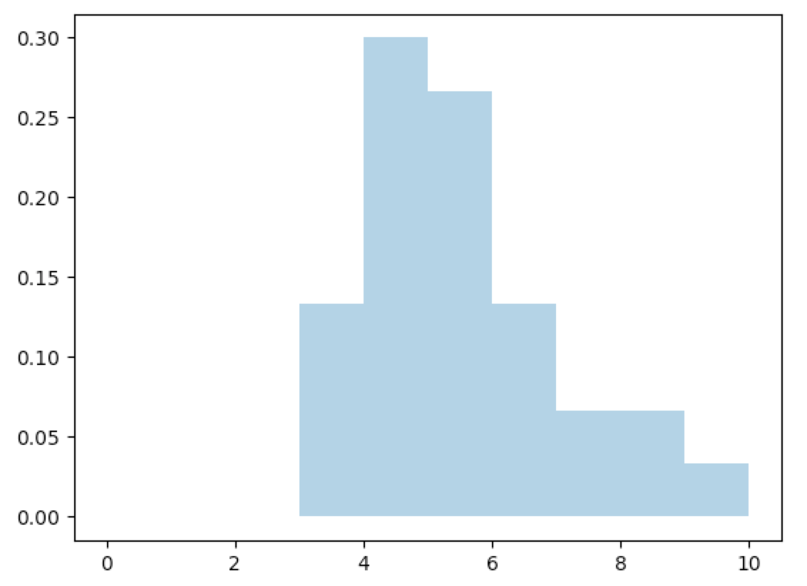
The data in Out[16] is as follows: column $1$: frequency, column $2$: mass, and column $3$: for that number of heads. It is very helpful to view this frequency or mass/density data in a histogram:
In [55]: import matplotlib.pyplot as plt

In [56]: plt.fill_between([i[2] for i in fx],[i[1] for i in fx], step="post", alpha=0.4)
Out[56]: <matplotlib.collections.PolyCollection at 0x118d2d048>

In [57]: plt.show()
Now let’s suppose we are interested in the frequency of the occurrence of $7$ heads. That is, we want to know how often we will get $7$ heads when we flip $10$ times. Let $X_i$ equal $1$ if trial $i$ resulted in $7$ heads, otherwise $0$. Then the Strong Law of Large Numbers tells us that with probability $1$:
$$ \lim_{n\goesto\infty}\frac{X_1+\dots+X_n}n\goesto\E{X_i}=\prt{7 heads in 10 flips}=\binom{10}7\fracpB12^7\fracpB12^3 \tag{LoLN.1} $$
The last equality follows because this is a binomial random variable. Hence the long run average frequency of getting $7$ heads in $10$ flips is $\binom{10}7\frac1{2^{10}}$.
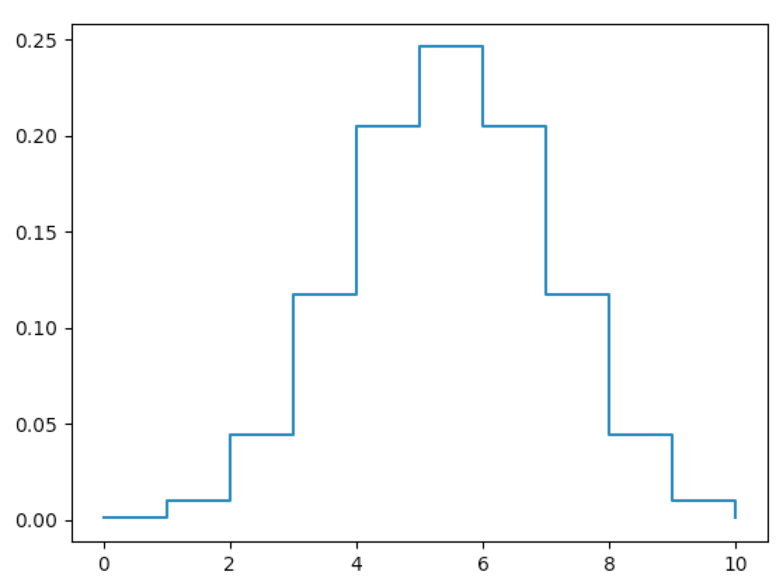
Now suppose we are interested in the long-run average frequency for all possible values $j=0,1,…,10$. This is the mass function of the binomial random variable with parameters $n=10$, $p=\frac12$:
In [17]: from sympy import binomial as binom, N

In [18]: winom=lambda n,i: N(binom(n,i))

In [19]: from numpy import power as pw

In [20]: brv=lambda n=10,i=0,p=1/2:winom(n,i)*pw(p,i)*pw(1-p,n-i)

In [21]: bx=[(float(brv(n=10,i=j,p=1/2)),j) for j in range(11)]

In [22]: bx
Out[22]:
[(0.0009765625, 0),
 (0.009765625, 1),
 (0.0439453125, 2),
 (0.1171875, 3),
 (0.205078125, 4),
 (0.24609375, 5),
 (0.205078125, 6),
 (0.1171875, 7),
 (0.0439453125, 8),
 (0.009765625, 9),
 (0.0009765625, 10)]

In [26]: plt.step([i[1] for i in bx],[i[0] for i in bx],where='post')
Out[26]: [<matplotlib.lines.Line2D at 0x1103f0dd8>]

In [27]: plt.show()
For any fixed $0\leq j\leq10$, define $X_i$ equal to $1$ if the $i^{th}$ trial resulted in $j$ heads, otherwise $0$. As in equation LoLN.1, we note that the SLoLN gives
$$ \lim_{n\goesto\infty}\frac{X_1+\dots+X_n}n\goesto\E{X_i}=\prt{j heads in 10 flips}=\binom{10}j\fracpB12^j\fracpB12^{10-j} $$
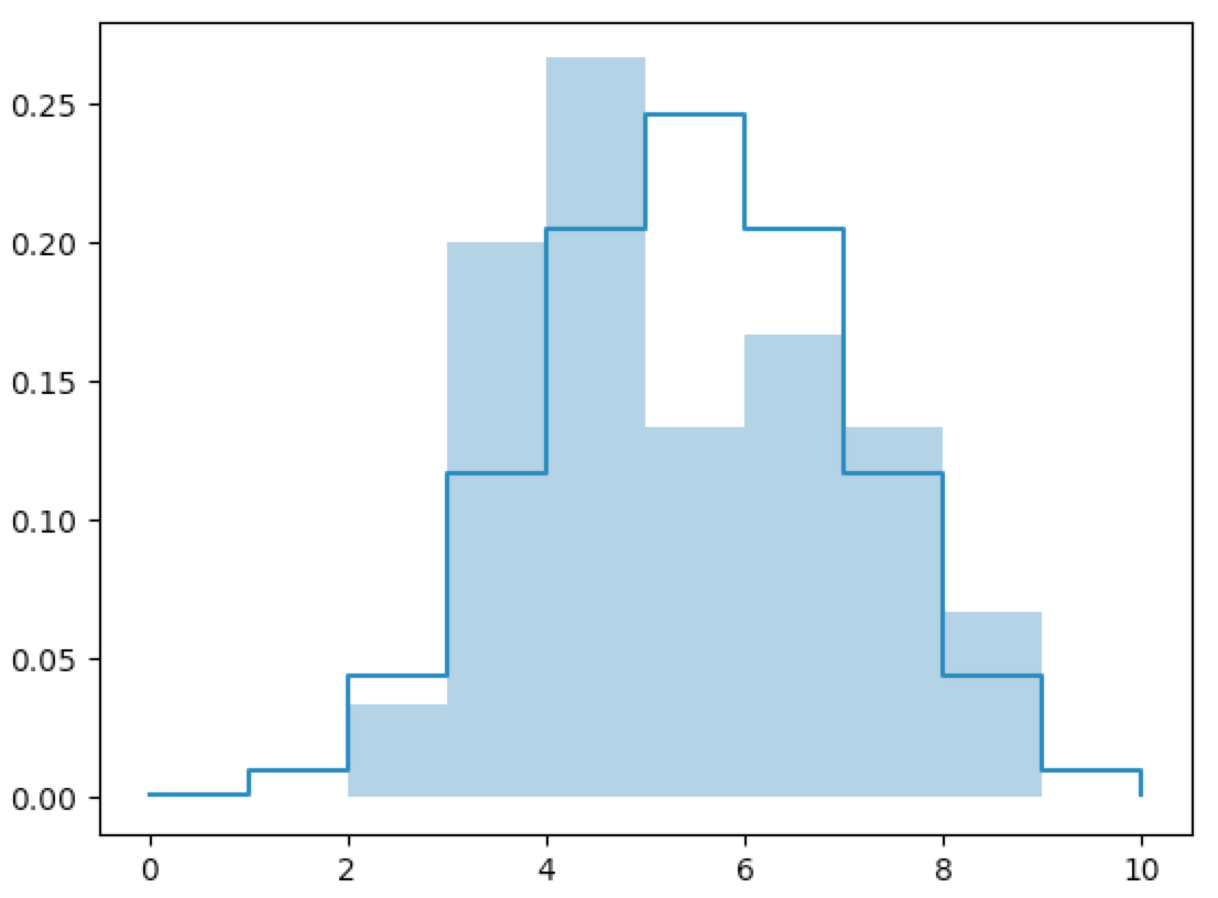
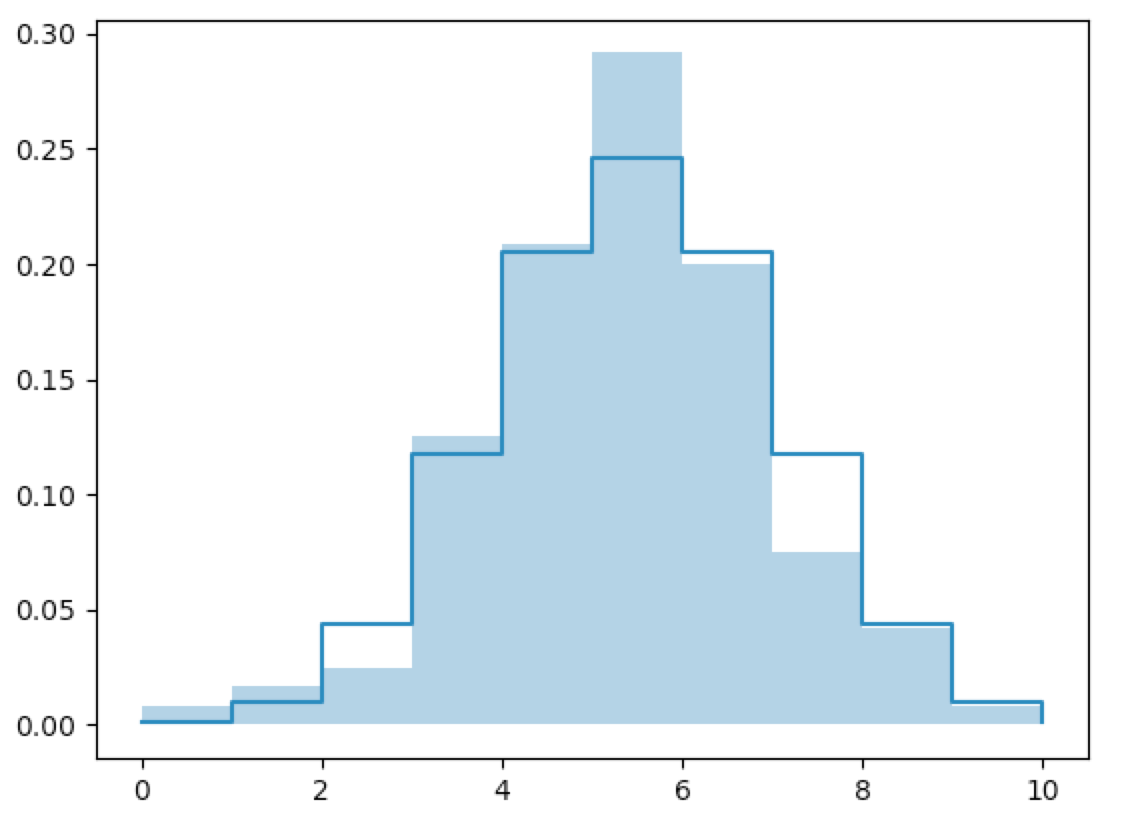
That is, the density histogram will converge to the mass function as $n\goesto\infty$:
In [60]: fx=flip_10_n(n=30)

In [61]: plt.step([i[1] for i in bx],[i[0] for i in bx],where='post')
Out[61]: [<matplotlib.lines.Line2D at 0x11a6286a0>]

In [62]: plt.fill_between([i[2] for i in fx],[i[1] for i in fx], step="post", alpha=0.4)
Out[62]: <matplotlib.collections.PolyCollection at 0x11a631a20>

In [63]: plt.show()

In [64]: fx
Out[64]:
[(0, 0.0, 0),
 (0, 0.0, 1),
 (1, 0.03333333333333333, 2),
 (6, 0.2, 3),
 (8, 0.26666666666666666, 4),
 (4, 0.13333333333333333, 5),
 (5, 0.16666666666666666, 6),
 (4, 0.13333333333333333, 7),
 (2, 0.06666666666666667, 8),
 (0, 0.0, 9),
 (0, 0.0, 10)]
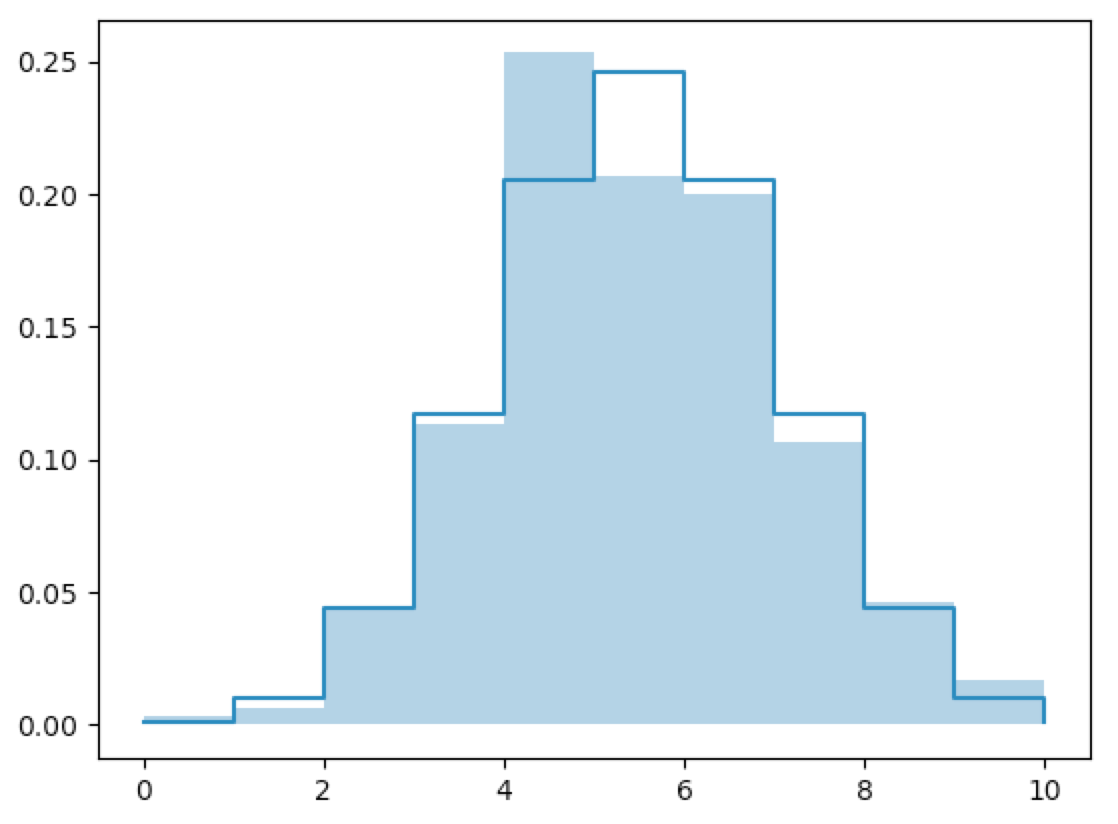
In [70]: fx=flip_10_n(n=60)

In [71]: fx
Out[71]:
[(0, 0.0, 0),
 (1, 0.016666666666666666, 1),
 (3, 0.05, 2),
 (10, 0.16666666666666666, 3),
 (9, 0.15, 4),
 (13, 0.21666666666666667, 5),
 (12, 0.2, 6),
 (9, 0.15, 7),
 (2, 0.03333333333333333, 8),
 (1, 0.016666666666666666, 9),
 (0, 0.0, 10)]
In [75]: fx=flip_10_n(n=120)

In [76]: fx
Out[76]:
[(1, 0.008333333333333333, 0),
 (2, 0.016666666666666666, 1),
 (3, 0.025, 2),
 (15, 0.125, 3),
 (25, 0.20833333333333334, 4),
 (35, 0.2916666666666667, 5),
 (24, 0.2, 6),
 (9, 0.075, 7),
 (5, 0.041666666666666664, 8),
 (1, 0.008333333333333333, 9),
 (0, 0.0, 10)]
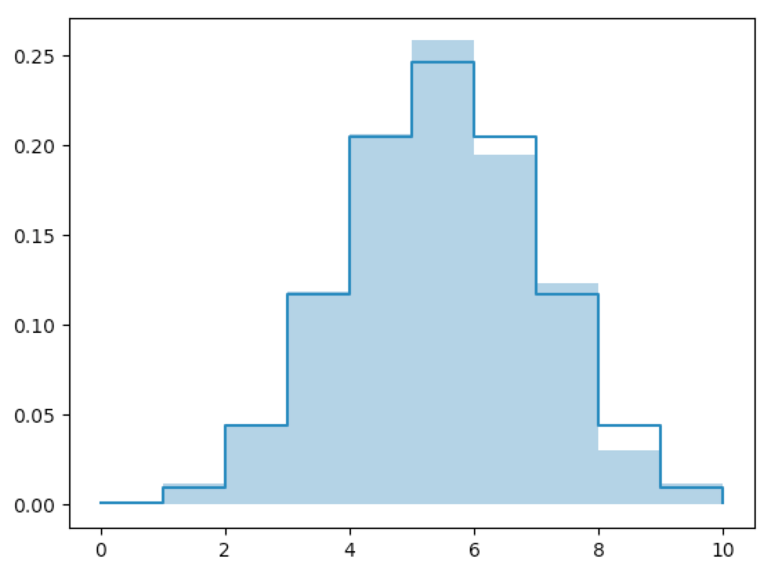
In [65]: fx=flip_10_n(n=300)

In [69]: fx
Out[69]:
[(1, 0.0033333333333333335, 0),
 (2, 0.006666666666666667, 1),
 (13, 0.043333333333333335, 2),
 (34, 0.11333333333333333, 3),
 (76, 0.25333333333333335, 4),
 (62, 0.20666666666666667, 5),
 (60, 0.2, 6),
 (32, 0.10666666666666667, 7),
 (14, 0.04666666666666667, 8),
 (5, 0.016666666666666666, 9),
 (1, 0.0033333333333333335, 10)]
In [80]: fx=flip_10_n(n=600)

In [81]: fx
Out[81]:
[(0, 0.0, 0),
 (7, 0.011666666666666667, 1),
 (27, 0.045, 2),
 (71, 0.11833333333333333, 3),
 (124, 0.20666666666666667, 4),
 (155, 0.25833333333333336, 5),
 (117, 0.195, 6),
 (74, 0.12333333333333334, 7),
 (18, 0.03, 8),
 (7, 0.011666666666666667, 9),
 (0, 0.0, 10)]
In [85]: fx=flip_10_n(n=6000)

In [86]: fx
Out[86]:
[(8, 0.0013333333333333333, 0),
 (37, 0.006166666666666667, 1),
 (267, 0.0445, 2),
 (688, 0.11466666666666667, 3),
 (1246, 0.20766666666666667, 4),
 (1481, 0.24683333333333332, 5),
 (1253, 0.20883333333333334, 6),
 (689, 0.11483333333333333, 7),
 (265, 0.04416666666666667, 8),
 (61, 0.010166666666666666, 9),
 (5, 0.0008333333333333334, 10)]
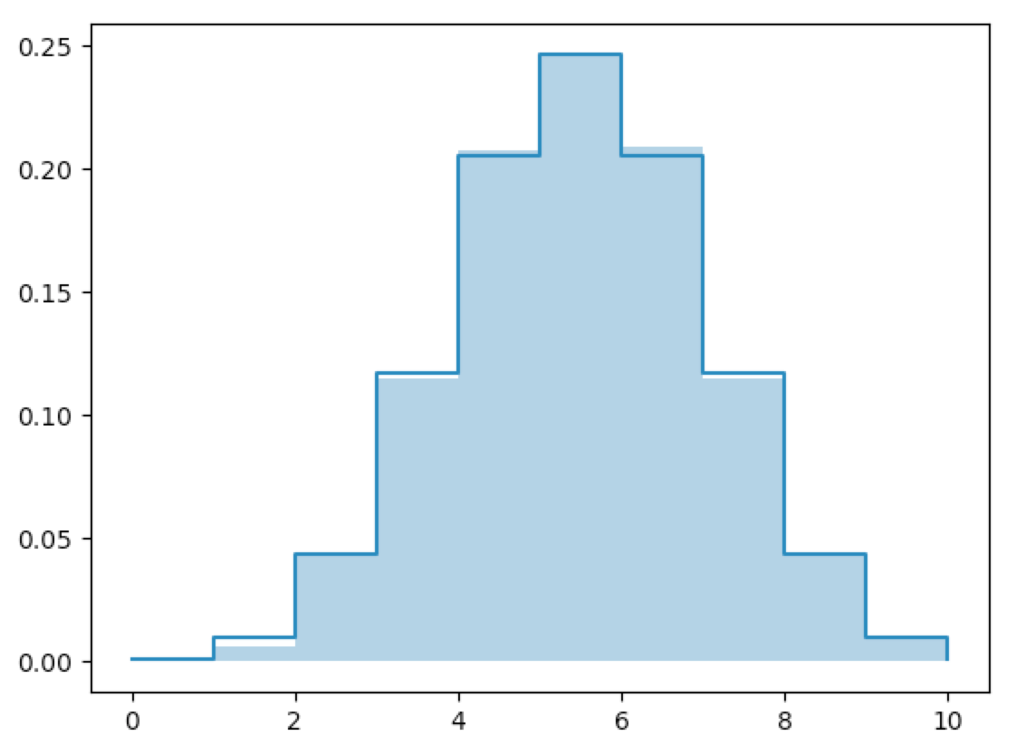
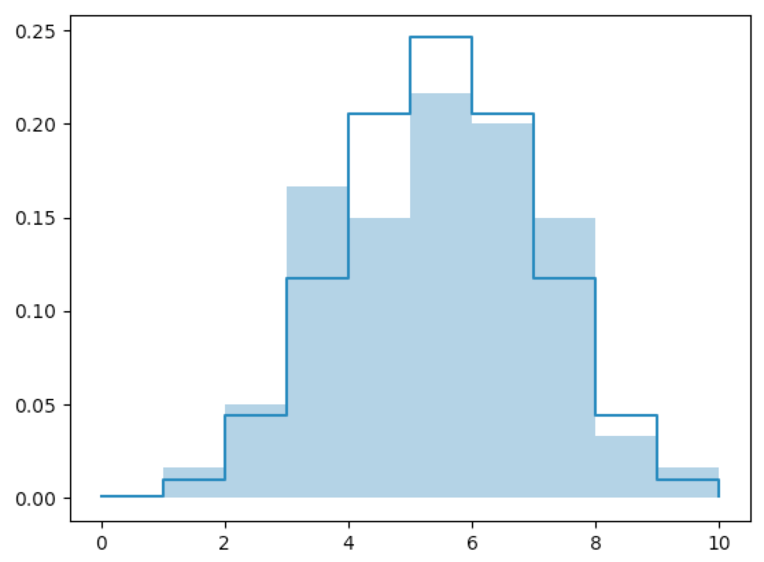
It should be clear that the mass histograms converge to the mass functions.
The LoLN can be applied to continuous random data as well. Let’s generate some data from an exponential distribution and see how it compares to the exponential density function:
In [143]: import seaborn as sns
In [144]: exp_dens=lambda lam=3,x=1:lam*np.exp(-lam*x)
In [145]: x=np.random.exponential(1/3,100)
In [146]: w=np.linspace(0,7,3000)
In [147]: y=exp_dens(lam=3,x=w)
In [148]: sns.distplot(x,kde=False,norm_hist=True)
Out[148]: <matplotlib.axes._subplots.AxesSubplot at 0x12f6d7d68>
In [149]: plt.plot(w, y)
Out[149]: [<matplotlib.lines.Line2D at 0x12f6a8e80>]
In [150]: plt.show()
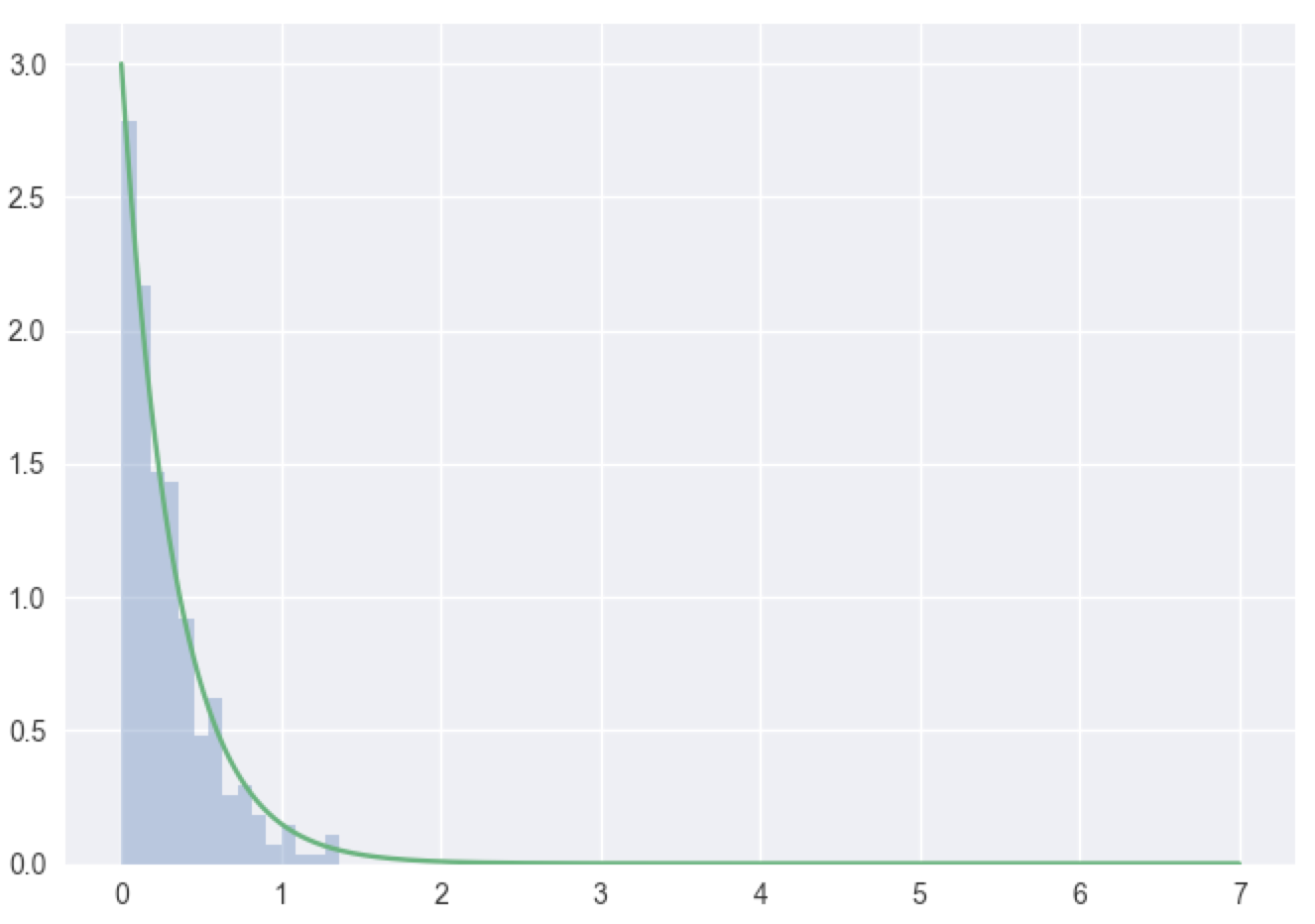
In [151]: x=np.random.exponential(1/3,300)
In [152]: sns.distplot(x,kde=False,norm_hist=True)
Out[152]: <matplotlib.axes._subplots.AxesSubplot at 0x13089d048>
In [153]: plt.plot(w, y)
Out[153]: [<matplotlib.lines.Line2D at 0x12d24d550>]
In [154]: plt.show()
In [155]: x=np.random.exponential(1/3,1000)
In [156]: sns.distplot(x,kde=False,norm_hist=True)
Out[156]: <matplotlib.axes._subplots.AxesSubplot at 0x13245c1d0>
In [157]: plt.plot(w, y)
Out[157]: [<matplotlib.lines.Line2D at 0x131a82da0>]
In [158]: plt.show()
In [159]: x=np.random.exponential(1/3,3000)
In [160]: sns.distplot(x,kde=False,norm_hist=True)
Out[160]: <matplotlib.axes._subplots.AxesSubplot at 0x132cc6198>
In [161]: plt.plot(w, y)
Out[161]: [<matplotlib.lines.Line2D at 0x131a8e4e0>]
In [162]: plt.show()
In [163]: x=np.random.exponential(1/3,10000)
In [164]: sns.distplot(x,kde=False,norm_hist=True)
Out[164]: <matplotlib.axes._subplots.AxesSubplot at 0x133f50630>
In [165]: plt.plot(w, y)
Out[165]: [<matplotlib.lines.Line2D at 0x134798cf8>]
In [166]: plt.show()
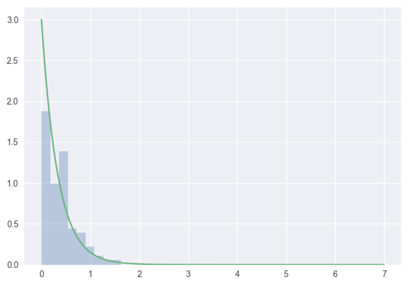
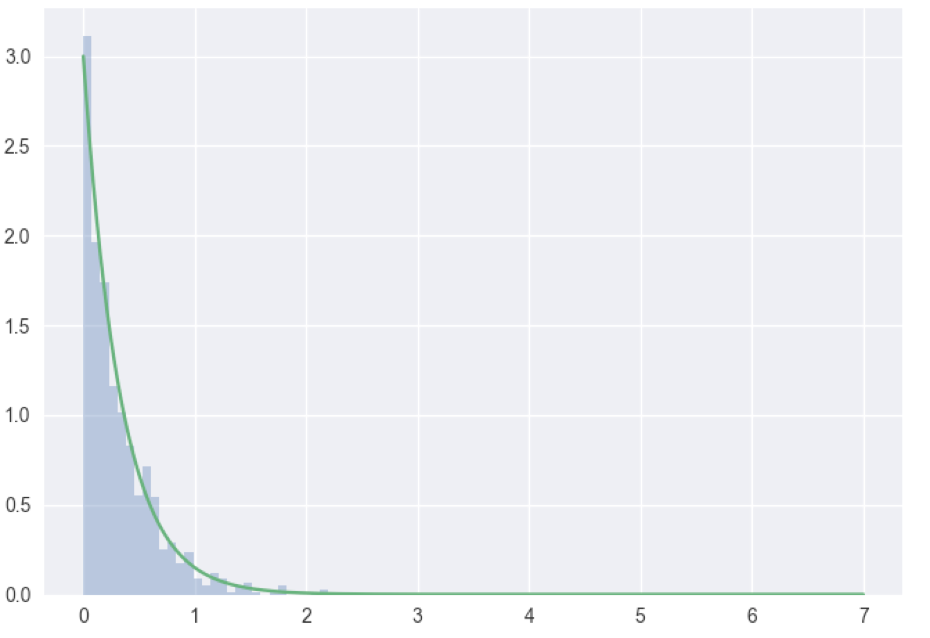

Again, the LoLN dictates that the mass histograms will converge to the density function.