The Problem
Suppose we have a coin but we don’t know if it’s fair or biased. So we flip the coin $10$ times and we get $7$ heads. What is the probability that the coin is biased for heads? What is the probability that we will get two heads in a row if we flip the coin two more times?
Bayesian
Let $\Theta$ denote the probability that the coin lands on heads. That is, if $C$ denotes the outcome of flipping the coin, then $\Theta\equiv\pr{C=h}$.
In Bayesian analysis, $\Theta$ is a random variable. This may seem strange since $\Theta\equiv\pr{C=h}$ is a fixed number. But Bayesians treat unknown quantities as random variables. This is the defining characteristic of Bayesian analysis.
Also let $N_n$ denote the number of heads in $n$ flips. Then we have
$$ \pdfa{\theta|i}{\Theta|N_n}=\frac{\cp{N_n=i}{\Theta=\theta}\pdfa{\theta}{\Theta}}{\pr{N_n=i}} \tag{B.1} $$
The proof and discussion for B.1 can be found in Ross, ch.6, p.267-268 and in my ch.6 notes. The probability in the numerator is
$$ \cp{N_n=i}{\Theta=\theta}=\binom{n}i\theta^i(1-\theta)^{n-i} $$
and the probability in the denominator is
$$ \pr{N_n=i}=\int_0^1\cp{N_n=i}{\Theta=\alpha}\pdfa{\alpha}{\Theta}d\alpha $$
This equality follows from Ross, p.344, section 7.5.3, equation 5.8.
If we know the distribution of $\Theta$, then we proceed. If not, then we must try to determine this. Suppose we have no idea what the distribution of the coin might be. In this case, it’s reasonable to assume a uniform distribution on $[0,1]$ (aka, flat prior). Then
$$ \pr{N_n=i}=\int_0^1\cp{N_n=i}{\Theta=\alpha}\wt1d\alpha=\int_0^1\binom{n}i\alpha^i(1-\alpha)^{n-i}d\alpha=\binom{n}i\frac{i!(n-i)!}{(n+1)!} \tag{B.2} $$
In the last equality, we made use of a property of the Beta Function. The useful property says that, for any positive integers $a$ and $b$, we have
$$ B(a.b)\equiv\int_0^1x^{a-1}(1-x)^{b-1}dx=\frac{(a-1)!(b-1)!}{(a+b-1)!} $$
To see the last equality in B.2, we set $a=i+1$ and $b=n-i+1$. Then $a-1=i$, $b-1=n-i$, and $a+b-1=i+1+n-i=n+1$. Hence
$$ \pr{N_n=i}=\binom{n}i\frac{i!(n-i)!}{(n+1)!}=\frac{n!}{i!(n-i)!}\frac{i!(n-i)!}{(n+1)!}=\frac{n!}{(n+1)!}=\frac1{n+1} $$
Putting it all together, we have
$$ \pdfa{\theta|i}{\Theta|N_n}=\frac{\cp{N_n=i}{\Theta=\theta}\pdfa{\theta}{\Theta}}{\pr{N_n=i}}=\frac{\binom{n}i\theta^i(1-\theta)^{n-i}}{\frac1{n+1}}=(n+1)\binom{n}i\theta^i(1-\theta)^{n-i} \tag{B.3} $$
Now we can compute:
$$ \prB{\Theta>\frac12}=\int_{\frac12}^1\pdfa{\theta}{\Theta}d\theta=\frac12 $$
and, for even $n$, we have
$$ \cpB{\Theta>\frac12}{N_{n}=\frac{n}2}=\int_{\frac12}^1\pdfab{\theta|\frac{n}2}{\Theta|N_{n}}d\theta=(n+1)\binom{n}{\frac{n}2}\int_{\frac12}^1\theta^{\frac{n}2}(1-\theta)^{n-\frac{n}2}d\theta $$
$$ =(n+1)\binom{n}{\frac{n}2}\int_{\frac12}^1\theta^{\frac{n}2}(1-\theta)^{\frac{n}2}d\theta \tag{B.4} $$
We perform this substitution in the integral:
$$ x=1-\theta\dq \theta=1-x\dq d\theta=-dx $$
$$ x_0=1-\theta_0=1-\frac12=\frac12\dq x_1=1-\theta_1=1-1=0 $$
To get
$$ \int_{\frac12}^1\theta^{\frac{n}2}(1-\theta)^{\frac{n}2}d\theta=-\int_{\frac12}^0(1-x)^{\frac{n}2}x^{\frac{n}2}dx=\int_0^{\frac12}(1-x)^{\frac{n}2}x^{\frac{n}2}dx $$
Hence
$$ 2\int_{\frac12}^1\theta^{\frac{n}2}(1-\theta)^{\frac{n}2}d\theta=\int_0^{\frac12}\theta^{\frac{n}2}(1-\theta)^{\frac{n}2}d\theta+\int_{\frac12}^1\theta^{\frac{n}2}(1-\theta)^{\frac{n}2}d\theta $$
$$ =\int_0^1\theta^{\frac{n}2}(1-\theta)^{\frac{n}2}d\theta=\frac{\fracpb{n}2!\fracpb{n}2!}{(n+1)!} $$
In the last equality, we again use the Beta function and we set $a=b=\frac{n}2+1$. Hence $a-1=b-1=\frac{n}2$ and $a+b-1=\frac{n}2+1+\frac{n}2=n+1$. Then B.4 becomes
$$ \cpB{\Theta>\frac12}{N_{n}=\frac{n}2}=(n+1)\binom{n}{\frac{n}2}\int_{\frac12}^1\theta^{\frac{n}2}(1-\theta)^{\frac{n}2}d\theta $$
$$ =\frac12(n+1)\binom{n}{\frac{n}2}\frac{\fracpb{n}2!\fracpb{n}2!}{(n+1)!}=\frac12(n+1)\frac{n!}{\fracpb{n}2!\prn{n-\frac{n}2}!}\frac{\fracpb{n}2!\fracpb{n}2!}{(n+1)!}=\frac12 $$
For example, if we flip the coin $10{,}000$ times and get $5{,}000$ heads, then it is just as likely that the coin favors heads as it is that the coin favors tails.
Now let’s solve our first original question: What is the probability that the coin is biased for heads?
$$ \cpB{\Theta>\frac12}{N_{10}=7}=\int_{\frac12}^1\pdfa{\theta|7}{\Theta|N_{10}}d\theta=11\binom{10}7\int_{\frac12}^1\theta^7(1-\theta)^3d\theta\approx0.887 $$
In [1]: from sympy import binomial as binom, N; from numpy import power as pw; import scipy.integrate

In [2]: winom=lambda n,i: N(binom(n,i))

In [3]: I=lambda f_x,a,b: scipy.integrate.quad(f_x,a,b)[0]

In [4]: tgn=lambda n=10,i=7: (n+1)*winom(n,i)*I(lambda t:pw(t,i)*pw(1-t,n-i),1/2,1)

In [5]: tgn()
Out[5]: 0.886718750000000

In [6]: tgn(n=100,i=70)
Out[6]: 0.999972334093724

In [7]: tgn(n=100,i=30)
Out[7]: 2.76653529378536e-5

In [8]: tgn(n=10,i=3)
Out[8]: 0.113281250000000
We can see from these computations that the more data we collect, the more confident we are in the coin’s bias. For example, when we flip the coin $10$ times and get $7$ heads, then there is a probability of $0.8867$ that the coin is biased to heads. But when we flip the coin $100$ times and get $70$ heads, then there is a probability of $0.9999$ that the coin is biased to heads.
Similarly, more data makes us more confident in the coin’s almost fairness:
In [54]: for n in [3,5,7,9,11,13,21,41,61,111,301,401,501,601,701,801,901,1001]:
...: i=int((n+1)/2)
...: print("n={} i={} tgn={}".format(n,i,tgn(n=n,i=i)))
...:
n=3 i=2 tgn=0.687500000000000
n=5 i=3 tgn=0.656250000000000
n=7 i=4 tgn=0.636718750000000
n=9 i=5 tgn=0.623046875000000
n=11 i=6 tgn=0.612792968750000
n=13 i=7 tgn=0.604736328125000
n=21 i=11 tgn=0.584094047546387
n=41 i=21 tgn=0.561192835623842
n=61 i=31 tgn=0.550461843173534
n=111 i=56 tgn=0.537612453152283
n=301 i=151 tgn=0.522937575457261
n=401 i=201 tgn=0.519885039957544
n=501 i=251 tgn=0.517796545193125
n=601 i=301 tgn=0.516253737036354
n=701 i=351 tgn=0.515051744901605
n=801 i=401 tgn=0.514082749436751
n=901 i=451 tgn=0.513279639144952
n=1001 i=501 tgn=0.512599917282251
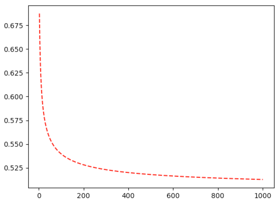
In [55]: def graph_tgn_near_half(n_range):
...: i_range=((n_range+1)/2).astype(int)
...: print("I_range={}".format(i_range))
...: y=[]
...: for n,i in zip(n_range,i_range):
...: y.append(tgn(n=n,i=i))
...: plt.plot(n_range,y,'r--')
...: plt.show()
...:
In [56]: graph_tgn_near_half(np.arange(3,1003,2))
Now let’s solve our second original question: What is the probability that we will get two heads in a row if we flip the coin two more times? Let’s again use equation 5.8 from Ross, p.344, section 7.5.3:
$$ \cp{(h,h)}{N_{10}=7}=\int_0^1\cp{(h,h)}{\Theta=\theta,N_{10}=7}\pdfa{\theta|7}{\Theta|N_{10}}d\theta $$
Now let’s assume conditional independence. That is, if $\Theta=\theta$ is given, then flip outcomes are independent. That is
$$ \cp{(h,h)}{\Theta=\theta,N_{10}=7}=\prn{\cp{(h)}{\Theta=\theta,N_{10}=7}}^2=\theta^2 $$
since the occurrence of $\Theta=\theta$ makes the occurrence of $N_{10}=7$ irrelevant. Hence
$$ \cp{(h,h)}{N_{10}=7}=11\binom{10}7\int_0^1\theta^2\theta^7(1-\theta)^3d\theta $$
In [61]: 11*winom(10,7)*I(lambda t:pw(t,9)*pw(1-t,3),0,1)
Out[61]: 0.461538461538462
We could also ask: what is the probability of exactly one head in the next two flips?
$$ \cptone{exactly 1 head in two flips}{N_{10}=7}=\cp{(h,t)}{N_{10}=7}+\cp{(t,h)}{N_{10}=7} $$
In [67]: 2*11*winom(10,7)*I(lambda t:pw(t,8)*pw(1-t,4),0,1)
Out[67]: 0.410256410256410
Or, what is the probability of no heads in the next two flips?
In [68]: 11*winom(10,7)*I(lambda t:pw(t,7)*pw(1-t,5),0,1)
Out[68]: 0.128205128205128
And a checksum:
In [69]: 11*winom(10,7)*I(lambda t:pw(t,9)*pw(1-t,3),0,1)+2*11*winom(10,7)*I(lambda t:pw(t,8)*pw(1-t,4),0,1)+11*winom(10,7)*I(lambda t
    ...: :pw(t,7)*pw(1-t,5),0,1)
Out[69]: 1.00000000000000
Lastly, we can ask, what is the probability of flipping a head with this coin, given that we flipped $7$ heads in $10$ flips?
$$ \cp{(h)}{N_{10}=7}=11\binom{10}7\int_0^1\theta\theta^7(1-\theta)^3d\theta=\frac23 \tag{B.5} $$
In [70]: 11*winom(10,7)*I(lambda t:pw(t,8)*pw(1-t,3),0,1)
Out[70]: 0.666666666666667
Bayesian Estimates
Now that we have some intuition into Bayesian statistics, let’s formally introduce some Bayesian estimates.
Bayesian MAP
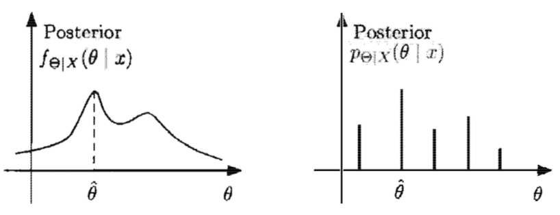
First we introduce the Maximum a Posteriori probability rule (MAP). For random variables $\Theta$ and $X$ and observation $X=x$, we have
$$ \hat{\theta}=\cases{\argmax{\theta}\cp{\Theta=\theta}{X=x}&\Theta\text{ discrete}\\\argmax{\theta}\pdfa{\theta|x}{\Theta|X}&\Theta\text{ continuous}} $$
Intuitively, we’re saying this: Let’s assume that our randomly observed data $x$ is representative of the population. Then it makes sense to estimate $\Theta$ with a value $\hat{\theta}$ that maximizes the probability that $\Theta=\theta$ given the realized data $x$.
Geometrically, we’re locating the maxima:
The form of the posterior distribution, as given by Bayes’ rule, provides an important computational shortcut: the denominator is the same for all $\theta$ and depends only on the value $x$ of the observation. That is, since
$$ \cp{\Theta=\theta}{X=x}=\frac{\pr{\Theta=\theta}\cp{X=x}{\Theta=\theta}}{\pr{X=x}} $$
then, for a given observation $X=x$, the denominator $\pr{X=x}$ is the same for all possible values of $\theta$. Hence when computing the maxima, we can disregard the denominator.
Thus, to maximize the posterior, we only need to choose a value of $\theta$ that maximizes the numerator $\pr{\Theta=\theta}\cp{X=x}{\Theta=\theta}$ if $\Theta$ and $X$ are discrete, or similar expressions if $\Theta$ and/or $X$ are continuous:
$$ \ht=\cases{\argmax{\theta}\pr{\Theta=\theta}\cp{X=x}{\Theta=\theta}&\Theta,X\text{ discrete}\\\argmax{\theta}\pr{\Theta=\theta}\pdfa{x|\theta}{X|\Theta}&\Theta\text{ discrete},X\text{ continuous}\\\argmax{\theta}\pdfa{\theta}{\Theta}\cp{X=x}{\Theta=\theta}&\Theta\text{ continuous},X\text{ discrete}\\\argmax{\theta}\pdfa{\theta}{\Theta}\pdfa{x|\theta}{X|\Theta}&\Theta,X\text{ continuous}} \tag{BMAP.1} $$
Now let’s find the MAP estimate from our example. From B.3, we have:
$$ \hat{\theta}=\argmax{\theta}\pdfa{\theta|i}{\Theta|N_n}=\argmax{\theta}(n+1)\binom{n}i\theta^i(1-\theta)^{n-i} $$
$$ =\argmax{\theta}\theta^i(1-\theta)^{n-i} $$
To maximize in $\theta$, we set the derivative to zero and solve for $\hat{\theta}$:
$$ 0=\wderiv{\sbr{\theta^i(1-\theta)^{n-i}}}{\theta}\eval{\hat{\theta}}{}=i\hat{\theta}^{i-1}(1-\hat{\theta})^{n-i}-\hat{\theta}^i(n-i)(1-\hat{\theta})^{n-i-1} $$
$\iff$
$$ (n-i)\hat{\theta}^i(1-\hat{\theta})^{n-i-1}=i\hat{\theta}^{i-1}(1-\hat{\theta})^{n-i} $$
$\iff$
$$ \frac{(n-i)\hat{\theta}^i(1-\hat{\theta})^{n-i-1}}{(n-i)\hat{\theta}^{i-1}(1-\hat{\theta})^{n-i-1}}=\frac{i\hat{\theta}^{i-1}(1-\hat{\theta})^{n-i}}{(n-i)\hat{\theta}^{i-1}(1-\hat{\theta})^{n-i-1}} $$
$\iff$
$$ \hat{\theta}=\frac{i}{n-i}(1-\hat{\theta})=\frac{i}{n-i}-\frac{i}{n-i}\hat{\theta} $$
$\iff$
$$ \frac{n}{n-i}\hat{\theta}=\frac{n-i}{n-i}\hat{\theta}+\frac{i}{n-i}\hat{\theta}=\frac{i}{n-i}\iff n\hat{\theta}=i\iff\hat{\theta}=\frac{i}{n} \tag{BMAP.2} $$
With $n=10$ and $i=7$, we get $\ht=\frac{7}{10}$
Bayesian Least Mean Squares
The LMS estimate is the conditional expection given the observed value:
$$ \ht=\Ec{\Theta}{X=x}=\cases{\sum_\theta\theta\cp{\Theta=\theta}{X=x}&\Theta\text{ discrete}\\\int_{-\infty}^\infty\theta\pdfa{\theta|x}{\Theta|X}d\theta&\Theta\text{ continuous}} $$
In our coin flipping example, we have
$$ \ht=\Ec{\Theta}{N_n=i}=\int_0^1\theta\pdfa{\theta|i}{\Theta|N_n}d\theta $$
$$ =(n+1)\binom{n}i\int_0^1\theta^{i+1}(1-\theta)^{n-i}d\theta $$
$$ =(n+1)\frac{n!}{i!(n-i)!}\int_0^1\theta^{i+2-1}(1-\theta)^{n-i+1-1}d\theta $$
$$ =\frac{(n+1)!}{i!(n-i)!}B(i+2,n-i+1) $$
$$ =\frac{(n+1)!}{i!(n-i)!}\frac{(i+1)!(n-i)!}{(i+2+n-i+1-1)!} $$
$$ =\frac{(n+1)!}{1}\frac{i+1}{(2+n)!}=\frac{i+1}{n+2} \tag{BLMS.1} $$
With $n=10$ and $i=7$, we get $\ht=\frac{8}{12}=\frac23$. Notice that this estimate matches with $\cp{(h)}{N_{10}=7}$ that we computed in B.5. This is because
$$ \cp{(h)}{N_{10}=7}=\int_0^1\cp{(h)}{\Theta=\theta,N_{10}=7}\pdfa{\theta|7}{\Theta|N_{10}}d\theta $$
$$ =\int_0^1\theta\pdfa{\theta|7}{\Theta|N_{10}}d\theta=\Ec{\Theta}{N_{10}=7}=\ht $$
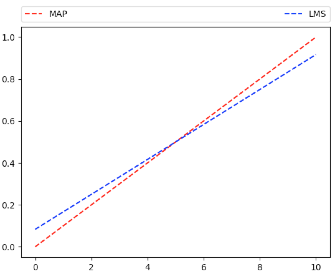
Let’s denote the MAP estimate by $\ht_{MAP}=\frac7{10}$ and let’s denote the Least Mean Squares estimate by $\ht_{LMS}=\frac23$. Now let’s plot $\ht_{MAP}$ and $\ht_{LMS}$ for $i=0,1,2,…,10$:
In [407]: thmap=lambda i=7,n=10: i/n

In [408]: thlms=lambda i=7,n=10: (i+1)/(n+2)

In [409]: def graph_ineff(funct, x_range, cl='r--', label=None, show=False):
     ...:     y_range=[]
     ...:     for x in x_range:
     ...:         y_range.append(funct(x))
     ...:     plt.plot(x_range,y_range,cl,label=label)
     ...:     if label is not None:
     ...:         plt.legend(bbox_to_anchor=(0., 1.02, 1., .102), loc=3,
     ...:            ncol=2, mode="expand", borderaxespad=0.)
     ...:     if show: plt.show()
     ...:

In [410]: graph_ineff(lambda i: thmap(i=i,n=10), range(0,11), label='MAP')

In [411]: graph_ineff(lambda i: thlms(i=i,n=10), range(0,11), cl='b--', label='LMS')

In [412]: plt.show()
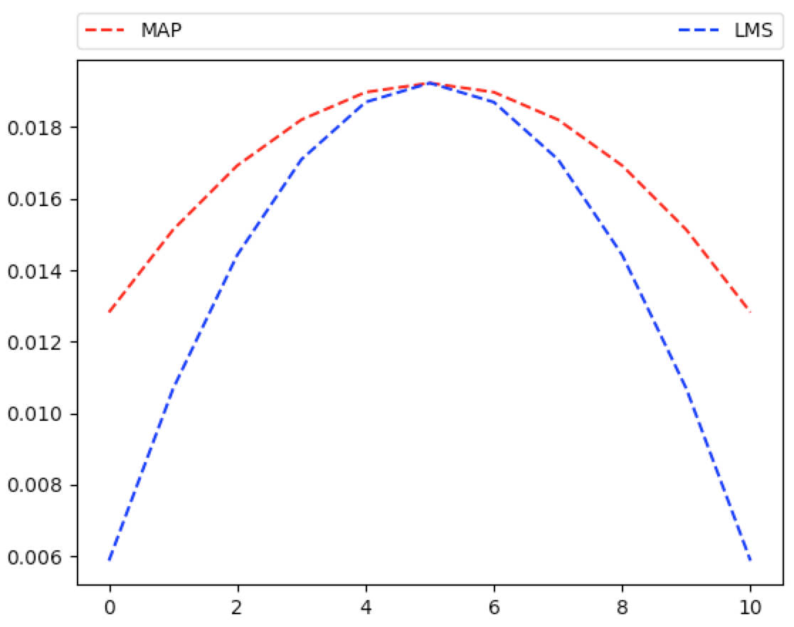
So which estimate is better? One possible measure for closeness to the actual distribution of $\Theta$ is the so-called Mean Squared Error (MSE): $\Ec{(\Theta-\ht)^2}{X=x}$. As you might guess by the titles, $\ht_{LMS}$ minimizes the MSE measurement.
You can find a proof of this in Ross, section 7.6, p.349-350, Proposition 6.1. Actually that proposition is for the uncondtional MSE. But inside this proof, the LMS is proven to minimize the conditional MSE. And Bertsekas-Tsitsiklis, p.431 nicely summarizes this.
We can compute the MSE for our example:
$$ \Ec{(\ht-\Theta)^2}{N_n=i}=\Ec{\ht^2-2\ht\Theta+\Theta^2}{N_n=i} $$
$$ =\Ec{\ht^2}{N_n=i}-\Ec{2\ht\Theta}{N_n=i}+\Ec{\Theta^2}{N_n=i} $$
$$ =\ht^2-2\ht\Ec{\Theta}{N_n=i}+\Ec{\Theta^2}{N_n=i} $$
$$ =\ht^2-2\ht\frac{i+1}{n+2}+\frac{(i+1)(i+2)}{(n+2)(n+3)} $$
where the last equation follows from a nice formula for the $m^{th}$ moment of a beta distribution, found on Bertsekas-Tsitsiklis, p.417 and then used on p.434.
And we can plot this:
In [427]: mse=lambda i=7,n=10,th=thmap:pw(th(i=i,n=n),2)-2*th(i=i,n=n)*(i+1)/(n+2)+(i+1)*(i+2)/((n+2)*(n+3))

In [428]: graph_ineff(lambda i: mse(i=i,n=10,th=thmap), range(0,11), label='MAP')

In [429]: graph_ineff(lambda i: mse(i=i,n=10,th=thlms), range(0,11), cl='b--', label='LMS')

In [430]: plt.show()
Frequentist
A frequentist would never regard $\Theta\equiv\pr{C=h}$ as a random variable since it is a fixed number. Instead, a frequentist would call this fixed number $\theta$ and try to estimate it. First let’s define the likelihood function.
Likelihood Function
For random variable $X$, observation $X=x$, and unknown, fixed parameter $\theta$, we define the PMF $\lfd{X}{x}{\theta}$ when $X$ is discete or PDF $\lfc{X}{x}{\theta}$ when $X$ is continuous. The form of each depends on the unknown $\theta$.
We refer to $\lfd{X}{x}{\theta}$ or $\lfc{X}{x}{\theta}$ as the likelihood function. In the event that $X=(X_1,…,X_n)$ is a vector and the observations $\set{X_i}$ are independent, then the likelihood function takes the form
$$ \lfd{X}{x_1,...,x_n}{\theta}=\prod_{i=1}^n\lfd{X_i}{x_i}{\theta}\dq\text{or}\dq\lfc{X}{x_1,...,x_n}{\theta}=\prod_{i=1}^n\lfc{X_i}{x_i}{\theta} $$
Let’s note a key distinction: having observed $X=x$, the functions $\lfd{X}{x}{\theta}$ or $\lfc{X}{x}{\theta}$ are NOT the probability that the unknown quantity is equal to $\theta$. Rather, each is the probability that the observed value $x$ occurs when the parameter (unknown constant) is equal to $\theta$.
Now, even though Frequentists view $\theta$ as an unknown constant, recall that Bayesians would call this $\Theta$ and regard it as a random variable. Then, if we assume that $\Theta$ is uniform, we may regard the likelihood function as a conditional probability:
$$ \lfd{X}{x}{\theta}=\cp{X=x}{\Theta=\theta}\dq\lfc{X}{x}{\theta}=\pdfa{x|\theta}{X|\Theta} \tag{F.1} $$
Before covering estimators, we quickly mention a modification of the likelihood function: the log likelihood function:
$$ \log\prn{\lfd{X}{x_1,...,x_n}{\theta}}=\log\Prn{\prod_{i=1}^n\lfd{X_i}{x_i}{\theta}}=\sum_{i=1}^n\log\prn{\lfd{X_i}{x_i}{\theta}} $$
or
$$ \log\prn{\lfc{X}{x_1,...,x_n}{\theta}}=\log\Prn{\prod_{i=1}^n\lfc{X_i}{x_i}{\theta}}=\sum_{i=1}^n\log\prn{\lfc{X_i}{x_i}{\theta}} $$
The log likelihood function is often convenient for analytical or computational reasons: we are generally interested in maximizing the likelihood function. Since the log function is strictly increasing, then the likelihood and log likelihood functions share maximum points.
Finding the maximum of a function often involves taking the derivative of a function and solving for the parameter being maximized. This is often easier todo with the log likelihood rather than likelihood function because the probability of joint, independent variables is the product of probabilities of the variables and solving an additive equation is usually easier than a multiplicative one.
Estimators
Now we define estimators: given observations $X=(X_1,…,X_n)$ that depend on an unknown constant $\theta$, an estimator is a random variable of the form $\hT=g(X)$, for some function $g$. Since the distribution of $X$ depends on $\theta$, so does the distribution of $\hT$. An actual realized value of $\hT$, denoted by $\ht$, is called an estimate.
One such estimate is the Maximum Likelihood Estimate (MLE): this is a value of the parameter $\theta$ that maximizes the numerical function $\lfd{X}{x}{\theta}$ or $\lfc{X}{x}{\theta}$ over all possible values of $\theta$:
$$ \hTmle\equiv\cases{\amt\lfd{X}{\wt}{\theta}&X\text{ discrete}\\\amt\lfc{X}{\wt}{\theta}&X\text{ continuous}} $$
$$ \htmle\equiv\cases{\amt\lfd{X}{x}{\theta}&X\text{ discrete}\\\amt\lfc{X}{x}{\theta}&X\text{ continuous}} \tag{F.2} $$
Note that $\hTmle=\amt\lfd{X}{\wt}{\theta}$ is a function of the unrealized observation $X$ and hence is an estimator whereas $\htmle=\amt\lfd{X}{x}{\theta}$ is a function of the realized observation $x$ and hence is an estimate. Also note that $\htmle$ is a numerical value.
Looking back at the Bayesian approach, let’s assume that $\Theta$ is flat (i.e. uniform). Then
$$ \pdfa{\theta}{\Theta}\cp{X=x}{\Theta=\theta}=c\cp{X=x}{\Theta=\theta} $$
for some positive constant $c$. Then we can disregard the constant when maximizing and BMAP.1 can be written as
$$ \htmap=\cases{\amt\cp{X=x}{\Theta=\theta}&X\text{ discrete}\\\amt\pdfa{x|\theta}{X|\Theta}&X\text{ continuous}} $$
Then F.1 and F.2 tell us that $\htmap=\htmle$ under the assumption that $\Theta$ is uniform.
Now let’s revisit the example: from BMAP.2, we have $\htmle=\htmap=\frac{i}{n}$ where $i$ is the number of heads observed in $n$ trials. Hence in our example, we have $\htmle=\frac7{10}$.
And the question: What is the probability that the coin is biased for heads? The frequentist would say the probability is $1$ since $\htmle=\htmap=\frac7{10}$ is a fixed number greater than $\frac12$. Recall that the Bayesian said this probability is $0.887$.
And the question: What is the probability that we will get two heads in a row if we flip the coin two more times? This is $\htmlesq=0.49\neq0.462\approx\cp{(h,h)}{N_{10}=7}$.
It’s interesting to compare the MLE estimate witht the LMS estimate from the Bayesian approach. Note again that $\htmle=\frac{i}n$, where $i$ is the number of heads observed in $n$ trials. And recall from BLMS.1 that the LMS estimate is $\frac{i+1}{n+2}$. The two estimates are similar but not identical. But they coincide asymptotically:
$$ \lim_{n\goesto\infty}\htmle=\lim_{n\goesto\infty}\frac{i}n=0=\lim_{n\goesto\infty}\frac{i+1}{n+2}=\lim_{n\goesto\infty}\htlms $$
Estimator Terminology And Properties
For a particular parameter of interest, let $\theta$ be the true, unknown constant value for that parameter.
Let $\hT_n$ be an estimator of $\theta$. That is, $\hT_n$ is a function of $n$ observations $X_1,…,X_n$ whose common distribution depends on $\theta$. That is, the observations $X=(X_1,…,X_n)$ are identically distributed and share the true, unknown constant $\theta$. Then define $\hT_n\equiv g(X)=g(X_1,…,X_n)$ for some function $g$.
The estimation error is $\tT_n\equiv\hT_n-\theta$ for the fixed, unknown $\theta$.
The bias of the estimator is the expected value of the estimation error:
$$ \biasTn\equiv\Ewrt{\theta}{\tT_n}=\Ewrt{\theta}{\hT_n}-\theta $$
Notice that the expected value of $\hT_n$ depends on the particular value $\theta$:
$$ \Ewrt{\theta}{\hT_n}=\cases{\sum_{\ht}\ht\lfd{\hT_n}{\ht}{\theta}&\hT_n\text{ discrete}\\\int\ht\lfc{\hT_n}{\ht}{\theta}d\ht&\hT_n\text{ continuous}} $$
Hence the bias also depends on the particular value $\theta$. Also note that the estimation error, expected value, and bias all depend on the unrealized observations $X_1,…,X_n$.
We say that $\hT_n$ is unbiased if $\Ewrt{\theta}{\hT_n}=\theta$ for every possible value of $\theta$.
We say that $\hT_n$ is asymptotically unbiased if $\lim_{n\goesto\infty}\Ewrt{\theta}{\hT_n}=\theta$ for every possible value of $\theta$.
We say that $\hT_n$ is consistent if the sequence $\hT_n$ converges to the true value of the parameter $\theta$, in probability, for every possible value of $\theta$.
These measures are helpful. But the MSE gives us the strongest quantitative measure of an estimator. Here’s an identity that comes up frequently and provides great intuition:
$$ MSE_{\theta}(\hT_n)=\Ewrt{\theta}{(\hT_n-\theta)^2}=\Vwrt{\theta}{\hT_n-\theta}+\prn{\Ewrt{\theta}{\hT_n-\theta}}^2=\Vwrt{\theta}{\hT_n}+\prn{\biasTn}^2 \tag{ETP.1} $$
That is, the MSE is the variance plus the square of the bias. Hence, to minimize MSE, we should try to minimize both variance and bias. But this is a balancing act that lies at the crux of machine learning.
Now let’s look again at our example. Let $\theta$ be the unknown probability of tossing heads and let $X_i$ be $1$ if the $i^{th}$ toss is heads, $0$ otherwise. Define the sample mean estimator:
$$ \hT_n\equiv\frac{X_1+\dots+X_n}{n}=\frac{N_n}n \tag{ETP.2} $$
Note that $\lfd{X_i}{1}{\theta}=\theta$ for all $i$. Hence, for any possible $\theta$, we have
$$ \Ewrt{\theta}{\hT_n}=\frac1n\sum_{i=1}^n\Ewrt{\theta}{X_i}=\frac1n\sum_{i=1}^n\lfd{X_i}{1}{\theta}=\frac1nn\theta=\theta \tag{ETP.3} $$
Hence $\hT_n$ is unbiased. And the SLoLN tells us that $\hT_n$ is also consistent since the $\set{X_i}$ are IID with mean $\theta$.
More generally, for IID $\set{X_i}$ with common variance $\sigma^2$, the sample mean estimate has variance
$$ \Vwrt{\theta}{\hT_n}=\frac1{n^2}\VBwrt{\theta}{\sum_{i=1}^nX_i}=\frac1{n^2}\sum_{i=1}^n\Vwrt{\theta}{X_i}=\frac1{n^2}\sum_{i=1}^n\sigma^2=\frac1{n^2}n\sigma^2=\frac{\sigma^2}n \tag{ETP.4} $$
Confidence Intervals
We are interested in constructing an interval that contains an unknown, fixed parameter value $\theta$ with a certain high probability, for every possible value of $\theta$.
More precisely, we first fix a desired confidence level, $1-\alpha$, where $\alpha$ is typically a small number. Then, from random observations $X_1,…,X_n$, we wish to find two point estimators, $\hT_n^-$ and $\hT_n^+$, such that $\hT_n^-\leq\hT_n^+$ and
$$ \prwrt{\theta}{\hT_n^-\leq\theta\leq\hT_n^+}\geq1-\alpha $$
That is, using the long run average frequency interpretation of probability, we wish to find point estimators $\hT_n^-$ and $\hT_n^+$ such that, over the long run, the realized point estimates $\ht_n^-$ and $\ht_n^+$ bracket the true value $\theta$ at least $1-\alpha$ percent of the time.
Said another way, each time we observe random data $X_1,…,X_n$, then there is a probability of at least $1-\alpha$ that the true value $\theta$ will be between the point estimators $\hT_n^-$ and $\hT_n^+$.
Note that $\hT_n^-$ and $\hT_n^+$ are functions of the observations. Hence they are random variables whose distributions depend on $\theta$. We call $[\hT_n^-,\hT_n^+]$ a $1-\alpha$ confidence interval.
Confidence intervals are usually constructed by forming an interval around the sample mean estimator $\hT_n$ in ETP.2. Then we use ETP.3, ETP.4, and the Central Limit Theorem to see that the CDF of the random variable
$$ \frac{\hT_n-\Ewrt{\theta}{\hT_n}}{\sqrt{\V{\hT_n}}}=\frac{\hT_n-\theta}{\sqrt{\frac{\sigma^2}{n}}}=\frac{\hT_n-\theta}{\frac{\sigma}{\sqrt{n}}} $$
approaches the standard normal CDF as $n$ increases, for every possible value of $\theta$.
We note that $\sqrt{\V{\hT_n}}=\frac\sigma{\sqrt{n}}$ is called the standard error. If we know the population variance, then this is a simple computation. If not, then we have a few options to estimate the true variance:
- Biased variance estimate of the sample mean: $\overline{S_n^2}=\frac1n\sum_{i=1}^n(X_i-\hT_n)^2$
- Unbiased variance estimate of the sample mean: $\hS_n^2=\frac1{n-1}\sum_{i=1}^n(X_i-\hT_n)^2$
- If the $\set{X_i}$ are Bernoulli: $\hat{\sigma}^2=\hT_n(1-\hT_n)$
- If the $\set{X_i}$ are Bernoulli: $\hat{\sigma}^2=\frac14$
(1) might be the most naturual but it can be shown to be biased (Bertsekas-Tsitsiklis p.467). (2) is unbiased. (3) is very computationally efficient. (4) is a nice conservative estimate since $\theta(1-\theta)$ for all $\theta\in[0,1]$.
Then we want to find $z$ such that
$$ 0.95=\prB{-z\leq\frac{\hT_n-\theta}{\sqrt{\Vwrt{\theta}{\hT_n}}}\leq z}=\prB{\frac{\norm{\hT_n-\theta}}{\sqrt{\Vwrt{\theta}{\hT_n}}}\leq z}=\prB{\frac{\norm{\theta-\hT_n}}{\sqrt{\Vwrt{\theta}{\hT_n}}}\leq z} $$
$$ \approx\prB{-z\leq\frac{\theta-\hT_n}{\frac{\hS_n}{\sqrt{n}}}\leq z}=\prB{-z\frac{\hS_n}{\sqrt{n}}\leq\theta-\hT_n\leq z\frac{\hS_n}{\sqrt{n}}} $$
$$ =\prB{\hT_n-z\frac{\hS_n}{\sqrt{n}}\leq\theta\leq\hT_n+z\frac{\hS_n}{\sqrt{n}}} $$
We set $\hT_n^-\equiv\hT_n-z\frac{\hS_n}{\sqrt{n}}$ and $\hT_n^+\equiv\hT_n+z\frac{\hS_n}{\sqrt{n}}$. And that’s our confidence interval.
Here is an implementation of a general confidence interval function with test script. It is helpful to review and experiment with these.