Example 8.5, p.418
$$ \pr{X_1=x_1,...,X_n=x_n}=\sum_{j=1}^2\cp{X_1=x_1,...,X_n=x_n}{\Theta=j}\pr{\Theta=j} $$
$$ =\sum_{j=1}^2\Sbr{\prod_{i=1}^n\cp{X_i=x_i}{\Theta=j}}\pr{\Theta=j} $$
$$ =\sum_{j=1}^2\pr{\Theta=j}\Sbr{\prod_{i=1}^n\cp{X_i=x_i}{\Theta=j}} $$
MAP, p.420
Define
$$ g_{MAP}(X=x)\equiv\wha{\theta}\equiv\argmax{\theta}\cp{\Theta=\theta}{X=x} $$
Then for fixed $x$ and fixed $\theta=g(x)$, we have
$$ \cp{g_{MAP}(X)=\Theta}{X=x}=\cp{g_{MAP}(X=x)=\Theta}{X=x} $$
$$ =\cp{\argmax{\theta'}\cp{\Theta=\theta'}{X=x}=\Theta}{X=x} $$
$$ =\cp{\wha{\theta}=\Theta}{X=x} $$
$$ \geq\cp{\theta=\Theta}{X=x} $$
$$ =\cp{g(X=x)=\Theta}{X=x} $$
Example 8.11, p.432
The joint PDF of $\Theta$ and $X$ is shown to be
$$ \pdfa{\theta,x}{\Theta,X}=\cases{\frac1{12}&4\leq\theta\leq10,\theta-1\leq x\leq\theta+1\\0&\text{otherwise}} $$
The support region can also be written as
$$ \pdfa{\theta,x}{\Theta,X}=\cases{\frac1{12}&3\leq x\leq11,\max(4,x-1)\leq\theta\leq\min(10,x+1)\\0&\text{otherwise}} $$
Confusing text: “Given that $X=x$, the posterior PDF $f_{\Theta\bar X}$ is uniform on the corresponding vertical section of the parallelogram.”
That is, suppose we observed $X=x_0\in[3,11]$. Then, for any $\theta\in[\max(4,x_0-1),\min(10,x_0+1)]$, we have
$$ \pdfa{\theta|x_0}{\Theta|X}=\frac{\pdfa{\theta,x_0}{\Theta,X}}{\pdfa{x_0}{X}}=\frac{\frac1{12}}{\pdfa{x_0}{X}}=c $$
where $c=\frac1{12\pdfa{x_0}{X}}$ is a constant relative to $\theta$. Similarly, for any $\theta<\max(4,x_0-1)$ or for any $\theta>\min(10,x_0+1)$, we have
$$ \pdfa{\theta|x_0}{\Theta|X}=\frac{\pdfa{\theta,x_0}{\Theta,X}}{\pdfa{x_0}{X}}=\frac{0}{\pdfa{x_0}{X}}=0 $$
Hence, for an observed, fixed $x_0\in[3,11]$, we have
$$ \pdfa{\theta|x_0}{\Theta|X}=\cases{c&\max(4,x_0-1)\leq\theta\leq\min(10,x_0+1)\\0&\text{otherwise}} $$
That is, $\set{\Theta\bar X=x_0}$ is uniform on $V_{x_0}\equiv\set{\theta:\theta\in[\max(4,x_0-1),\min(10,x_0+1)]}$. Note that the “corresponding vertical section of the parallelogram” is precisely the set $V_{x_0}$.
Next confusion: “Thus $\Ec{\Theta}{X=x}$ is the midpoint of that section”: First note that we can break out the $V_{x_0}$ like this
$$ V_{x_0}=\cases{\set{\theta:\theta\in[4,x_0+1]}&x_0\in[3,5]\\\set{\theta:\theta\in[x_0-1,x_0+1]}&x_0\in[5,9]\\\set{\theta:\theta\in[x_0-1,10]}&x_0\in[9,11]} $$
Recall the mean of a random variable that is uniform on $(\alpha,\beta)$: $\frac{\alpha+\beta}2$. Hence
$$ \Ec{\Theta}{X=x_0}=\cases{\frac{x_0+5}2&x_0\in[3,5]\\x_0&x_0\in[5,9]\\\frac{x_0+9}2&x_0\in[9,11]} \tag{Ex.8.11.1} $$
And these are just the midpoints of the vertical sections.
Next confusion: “which in this example happens to be a piecewise linear function of $x$.” Note that Ex.8.11.1 is a piecewise linear function of $x_0$.
Let’s also compute the conditional MSE and compare to the given graph:
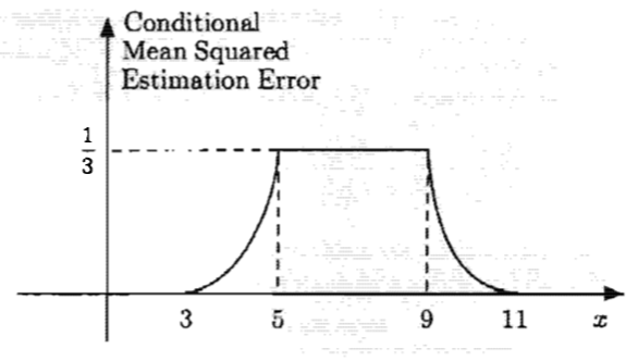
Note that
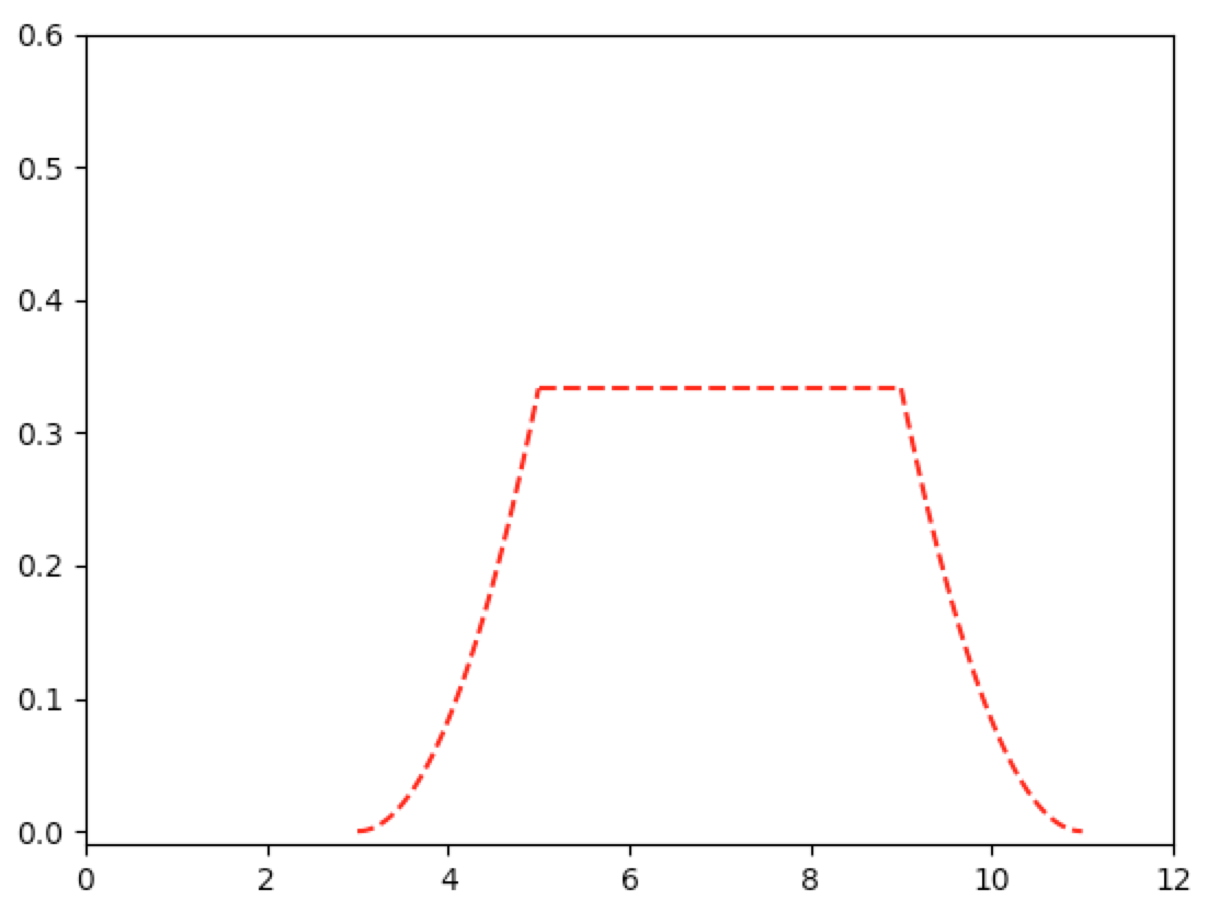
$$ \Ec{(\Theta-\Ec{\Theta}{X})^2}{X=x_0}=\Vc{\Theta}{X=x_0}=\cases{\frac{(x_0-3)^2}{12}&x_0\in[3,5]\\\frac{2^2}{12}&x_0\in[5,9]\\\frac{(11-x_0)^2}{12}&x_0\in[9,11]} $$
In [372]: from matplotlib import pyplot as plt

In [373]: def graph_ineff(funct, x_range, cl='r--', show=False):
     ...:     y_range=[]
     ...:     for x in x_range:
     ...:         y_range.append(funct(x))
     ...:     plt.plot(x_range,y_range,cl)
     ...:     if show: plt.show()
     ...:

In [374]: graph_ineff(lambda x: pw(x-3,2)/12, np.linspace(3,5,100))

In [375]: graph_ineff(lambda x: 1/3, np.linspace(5,9,100))

In [376]: graph_ineff(lambda x: pw(x-11,2)/12, np.linspace(9,11,100))

In [377]: plt.xlim(0,12)
Out[377]: (0, 12)

In [378]: plt.ylim(-0.01,3/5)
Out[378]: (-0.01, 0.6)

In [379]: plt.show()
Example 8.14, p.437
Let’s define
$$ \hat{\Theta}\equiv\Ec{\Theta}{X}\dq\dq\tilde{\Theta}\equiv\hat{\Theta}-\Theta $$
Since $\E{\tilde{\Theta}}=0$, we see that
$$ \V{\tilde{\Theta}}=\E{\tilde{\Theta}^2}-\prn{\E{\tilde{\Theta}}}^2=\E{\tilde{\Theta}^2} $$
Also, since $\V{\Theta}=\V{\hat{\Theta}}+\V{\tilde{\Theta}}$, then we have
$$ \E{\tilde{\Theta}^2}=\V{\tilde{\Theta}}=\V{\Theta}-\V{\hat{\Theta}} $$
Hence $\E{\tilde{\Theta}^2}=\V{\Theta}$ if and only if $\V{\hat{\Theta}}=0$. That is, the observation $X$ is uninformative if and only if $\V{\hat{\Theta}}=0$.
Quick Aside 1 A random variable is constant if and only if it’s equal to its mean.
Proof Let’s show that $Y$ is constant IFF $Y=\E{Y}$. If $Y=\E{Y}$, then $Y$ is clearly constant. In the other direction, suppose $Y=a$ for some number $a$. Then
$$ \E{Y}=\E{a}=a=Y $$
$\wes$
Quick Aside 2 The variance of a random variable is zero if and only if that variable is constant.
Proof Suppose $Y$ is constant. Then
$$ \V{Y}=\E{Y^2}-\prn{\E{Y}}^2=\Eb{\prn{\E{Y}}^2}-\prn{\E{Y}}^2=\prn{\E{Y}}^2-\prn{\E{Y}}^2=0 $$
Hence if $Y$ is constant, then $\V{Y}=0$. In the other direction, see Ross, Ch.8, Proposition 2.3, p.390.
$\wes$
Hence $X$ is uninformative if and only if $\hat{\Theta}=\E{\hat{\Theta}}$. But $\hat{\Theta}\equiv\Ec{\Theta}{X}$. Hence $X$ is uninformative if and only if, for every value of $X$, we have
$$ \Ec{\Theta}{X}=\hat{\Theta}=\E{\hat{\Theta}}=\E{\Ec{\Theta}{X}}=\E{\Theta} $$
Linear Least Mean Squares Estimation Based on a Single Observation, p.437-438
Define $Y_a=\Theta-aX$. And choose $b$ to be
$$ b\equiv\E{\Theta-aX}\equiv\E{Y_a} $$
With this choice of $b$, we wish to minimize
$$ \Eb{\prn{\Theta-aX-b}^2}=\Eb{\prn{Y_a-\E{Y_a}}^2}=\V{Y_a}=\V{\Theta-aX} $$
After solving for $a$, we want to know the MSE of the resulting linear estimator $\hat{\Theta}=aX+b$. The MSE of any estimator $\hat{\Theta}$ of $\Theta$ is
$$ \Eb{(\Theta-\hat{\Theta})^2}=\V{\Theta-\hat{\Theta}}+\prn{\E{\Theta-\hat{\Theta}}}^2 \tag{LLMS-SO-1} $$
In the case of this estimator $\hat{\Theta}=aX+b$, we have
$$ \E{\Theta-\hat{\Theta}}=\E{\Theta}-\E{\hat{\Theta}}=\E{\Theta}-\E{aX+b} $$
$$ =\E{\Theta}-\prn{a\E{X}+b}=\E{\Theta}-\prn{a\E{X}+\E{\Theta-aX}} $$
$$ =\E{\Theta}-a\E{X}-\E{\Theta-aX}=\E{\Theta}-a\E{X}-\E{\Theta}+a\E{X}=0 $$
Then LLMS-SO-1 becomes
$$ \Eb{(\Theta-\hat{\Theta})^2}=\V{\Theta-\hat{\Theta}}+\prn{\E{\Theta-\hat{\Theta}}}^2=\V{\Theta-\hat{\Theta}} $$
$$ =\V{\Theta-(aX+b)}=\V{\Theta-aX-b}=\V{\Theta-aX} $$
And here is a handy formula for $\hat{\Theta}$:
$$ \hat{\Theta}=aX+b=aX+\E{\Theta}-a\E{X}=\E{\Theta}+a\prn{X-\E{X}}=\E{\Theta}+\corr{\Theta}{X}\frac{\sigma_\Theta}{\sigma_X}\prn{X-\E{X}} $$
$$ =\E{\Theta}+\frac{\covw{\Theta}{X}}{\V{X}}\prn{X-\E{X}} $$
where
$$ \corr{\Theta}{X}=\frac{\covw{\Theta}{X}}{\sigma_\Theta\sigma_X}=\frac{\E{(\Theta-\E{\Theta})(X-\E{X})}}{\sigma_\Theta\sigma_X} $$
and
$$ \corr{\Theta}{X}\frac{\sigma_\Theta}{\sigma_X}=\frac{\covw{\Theta}{X}}{\sigma_\Theta\sigma_X}\frac{\sigma_\Theta}{\sigma_X}=\frac{\covw\Theta{X}}{\sigma_X^2} $$
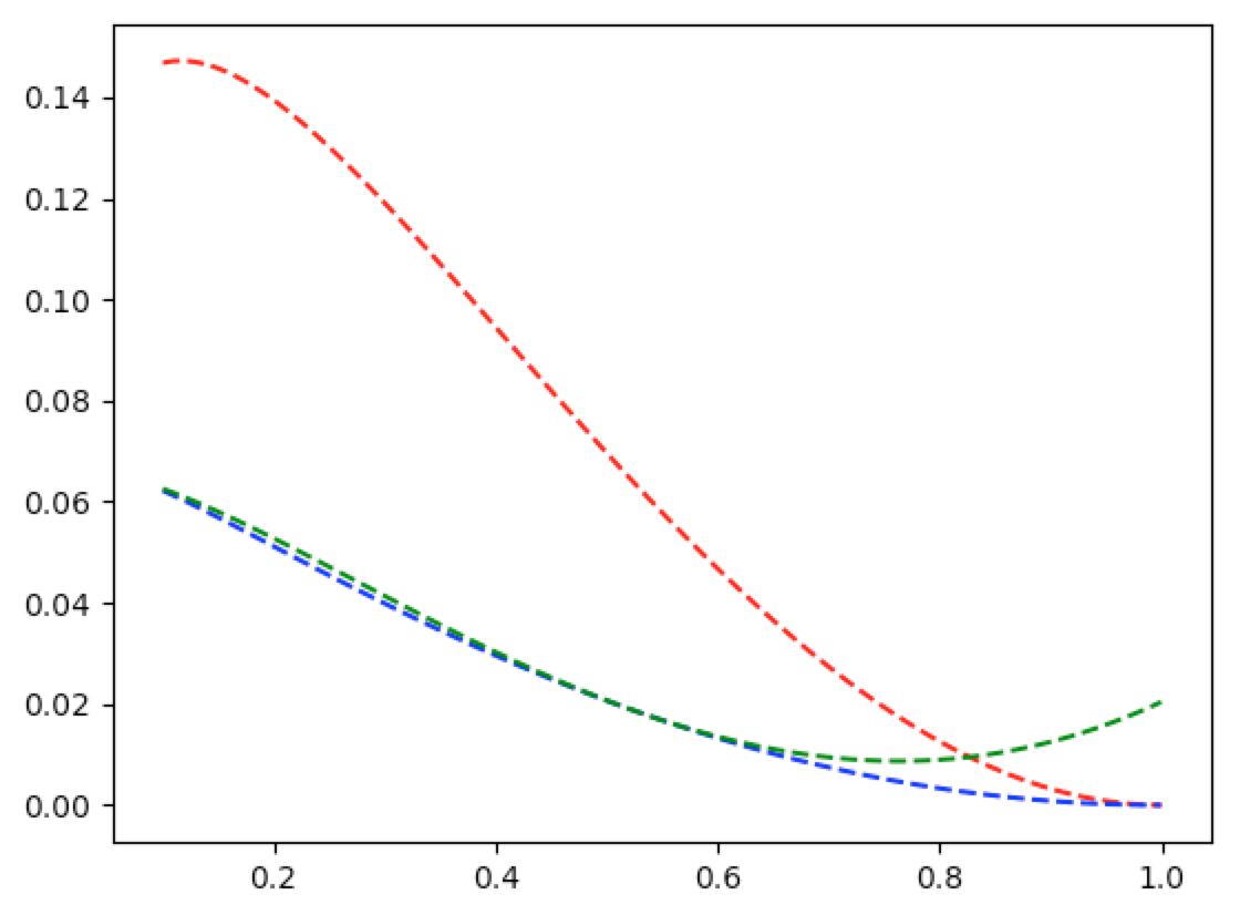
Example 8.15. p.440
In [359]: w1=lambda x=1/2: pw(x,2)+(3*pw(x,2)-4*x+1)/(2*np.abs(np.log(x)))

In [360]: w2=lambda x=1/2:(1-pw(x,2))/(2*np.abs(np.log(x)))-pw((1-x)/np.log(x),2)

In [361]: wt=lambda t=1/2,x=1/2: pw(t,2)-t*(2*(1-x))/np.abs(np.log(x))+(1-pw(x,2))/(2*np.abs(np.log(x)))

In [362]: w3=lambda x=1/2: wt(t=(6/7)*x+2/7,x=x)

In [363]: graph_ineff(lambda x: w1(x), np.linspace(0.1,0.9999,100))

In [364]: graph_ineff(lambda x: w2(x), np.linspace(0.1,0.9999,100), cl='b--')

In [365]: graph_ineff(lambda x: w3(x), np.linspace(0.1,0.9999,100), cl='g--')

In [366]: plt.show()