Before we start approximating functions, let’s first review a key property from orthogonal projection.
Key Property of Orthogonal Projection
Let $V$ be a inner product space over $\mathbb{C}$ or $\mathbb{R}$ and let $U$ be a finite-dimensional subspace of $V$. Then $V=U\oplus U^\perp$ (see Axler, Linear Alegbra Done Right, 6.47). Let $v\in V$ so that $v=u+w$ for some $u\in U$ and some $w\in U^\perp$. Let $P_Uv$ denote the orthogonal projection of $v$ into $U$. Hence $P_Uv=u$.
Let $e_1,\dots,e_m$ be an orthonormal basis of $U$. Then
$$\begin{align*} P_Uv &= u \\ &= \sum_{k=1}^m\innprd{u}{e_k}e_k\tag{by Axler, 6.30} \\ &= \sum_{k=1}^m\innprd{u}{e_k}e_k+\sum_{k=1}^m\innprd{w}{e_k}e_k \\ &= \sum_{k=1}^m\prn{\innprd{u}{e_k}+\innprd{w}{e_k}}e_k \\ &= \sum_{k=1}^m\innprd{u+w}{e_k}e_k \\ &= \sum_{k=1}^m\innprd{v}{e_k}e_k\tag{1} \end{align*}$$
The third equality holds because $w\in U^\perp$. Hence $\innprd{w}{e_k}=0$.
Approximation with Polynomials
The problem we want to look at is this: Let $v$ be a continuous real-valued function on some interval in $\mathbb{R}$. Can we find some polynomial (that would likely be easier to work with) that closely approximates $v$ on this interval? One way to measure the approximation error is
$$ \int_{a}^{b}\normw{v(t)-p(t)}^2dt $$
where $p$ is any approximating polynomial. So we can formulate our problem as follows. Let $\mathscr{P}_{\wR}[a,b]$ denote the vector space of real-valued polynomials on $[a,b]$. Find a polynomial $u\in\mathscr{P}_{\wR}[a,b]$ such that
$$ \int_{a}^{b}\normw{v(t)-u(t)}^2dt\leq\int_{a}^{b}\normw{v(t)-p(t)}^2dt\quad\text{for all }p\in\mathscr{P}_{\wR}[a,b] $$
Let’s look at an example. Let $v$ be the sine function and consider the interval $[-\pi,\pi]$. Let $\mathscr{C}_{\mathbb{R}}[-\pi,\pi]$ denote the real inner product space of continuous real-valued functions on $[-\pi,\pi]$ with inner product
$$ \innprd{f}{g}\equiv\int_{-\pi}^{\pi}f(t)g(t)dt $$
Let $U$ denote the subspace of $\mathscr{C}_{\mathbb{R}}[-\pi,\pi]$ consisting of polynomials with real coefficients and degree at most $5$. Then, for any $p\in U$, we have
$$ \dnorm{v-p}^2=\innprd{v-p}{v-p}=\int_{-\pi}^{\pi}(v-p)(t)(v-p)(t)dt=\int_{-\pi}^{\pi}\normw{v(t)-p(t)}^2dt $$
Hence our problem can be reformulated to finding $u\in U$ such that
$$ \dnorm{v-u}\leq\dnorm{v-p}\quad\text{for all }p\in U $$
That is, we want to minimize the distance from $v\in\mathscr{C}_{\wR}[-\pi,\pi]$ to the subspace $U$ by choosing $u\in U$ appropriately. To do this, we set $u\equiv P_Uv$ (by Axler 6.56). That is, for any $p\in U$, we have
$$ \dnorm{v-P_Uv}\leq\dnorm{v-p} $$
So we must compute $P_Uv$. Equation (1) from above gives us a formula for computing $P_Uv$. But we need an orthonormal basis of $U$ for this. Recall that $1,x,x^2,x^3,x^4,x^5$ is a basis of $U$. Let $e_0,e_1,e_2,e_3,e_4,e_5$ be the orthonormal basis given by applying Gram-Schmidt to the basis $1,x,x^2,x^3,x^4,x^5$ of $U$. Hence
$$ e_0\equiv\frac{1}{\dnorm{1}} \quad\quad\quad e_1\equiv\frac{x-\innprd{x}{e_0}e_0}{\dnorm{x-\innprd{x}{e_0}e_0}} \quad\quad\quad e_2\equiv\frac{x^2-\innprd{x^2}{e_0}e_0-\innprd{x^2}{e_1}e_1}{\dnorm{x^2-\innprd{x^2}{e_0}e_0-\innprd{x^2}{e_1}e_1}} $$
$$ e_3\equiv\frac{x^3-\sum_{j=0}^2\innprd{x^3}{e_j}e_j}{\dnorm{x^3-\sum_{j=0}^2\innprd{x^3}{e_j}e_j}} \quad\quad\quad e_4\equiv\frac{x^4-\sum_{j=0}^3\innprd{x^4}{e_j}e_j}{\dnorm{x^4-\sum_{j=0}^3\innprd{x^4}{e_j}e_j}} \quad\quad\quad e_5\equiv\frac{x^5-\sum_{j=0}^4\innprd{x^5}{e_j}e_j}{\dnorm{x^5-\sum_{j=0}^4\innprd{x^5}{e_j}e_j}} $$
So we compute
$$ \dnorm{1}=\sqrt{\innprd{1}{1}}=\sqrt{\int_{-\pi}^\pi1(t)\cdot1(t)dt}=\sqrt{t\eval{-\pi}{\pi}}=\sqrt{\pi--\pi}=\sqrt{2\pi} $$
and
$$ e_0\equiv\frac{1}{\dnorm{1}}=\frac1{\sqrt{2\pi}}1 $$
Next
$$\begin{align*} \innprd{x}{e_0} &= \innprd{x}{\frac1{\sqrt{2\pi}}1} \\ &= \int_{-\pi}^{\pi}x(t)\frac1{\sqrt{2\pi}}1(t)dt \\ &= \frac1{\sqrt{2\pi}}\int_{-\pi}^{\pi}tdt \\ &= \frac1{\sqrt{2\pi}}\frac12\Prn{t^2\eval{-\pi}{\pi}} \\ &= \frac1{\sqrt{2\pi}}\frac12\prn{\pi^2-(-\pi)^2} \\ &= 0 \end{align*}$$
and
$$\begin{align*} \dnorm{x}^2 &= \innprd{x}{x} \\ &= \int_{-\pi}^{\pi}x(t)x(t)dt \\ &= \int_{-\pi}^{\pi}t\cdot tdt \\ &= \int_{-\pi}^{\pi}t^2dt \\ &= \frac13\Prn{t^3\eval{-\pi}{\pi}} \\ &= \frac13\prn{\pi^3-(-\pi)^3} \\ &= \frac13\prn{\pi^3-(-1)^3\pi^3} \\ &= \frac13\prn{\pi^3+\pi^3} \\ &= \frac{2\pi^3}{3} \end{align*}$$
Hence
$$ e_1\equiv\frac{x-\innprd{x}{e_0}e_0}{\dnorm{x-\innprd{x}{e_0}e_0}}=\frac{x}{\dnorm{x}}=\frac{x}{\sqrt{\frac{2\pi^3}{3}}}=\sqrt{\frac{3}{2\pi^3}}x $$
We can compute the other $e_k$’s similarly. Then we can use (1) to compute the orthogonal projection:
$$\begin{align*} P_Uv &= \sum_{k=0}^5\innprd{v}{e_k}e_k \\ &= \sum_{k=0}^5\innprd{\sin}{e_k}e_k \\ &= \sum_{k=0}^5\Prn{\int_{-\pi}^{\pi}\sin{(t)}e_k(t)dt}e_k \\ \end{align*}$$
Let’s code this up:
import numpy as np
import scipy.integrate as integrate
import matplotlib.pyplot as plt

func_innprd=lambda f,g: integrate.quad(lambda t: f(t)*g(t),-np.pi,np.pi)[0]
func_norm=lambda f: np.sqrt(func_innprd(f,f))

polynomial_degree=13
def orig_basis_vec(i): return lambda t: t**i
orig_bis=[orig_basis_vec(i) for i in range(polynomial_degree+1)]
orth_bis={}
ips={}

def compute_inner_prods(k=5,degree=5):
    for i in range(k,degree+1):
        xi=orig_bis[i]
        ek=orth_bis[k]
        ips[(i,k)]=func_innprd(xi,ek)
    return

def gram_schmidt(k=5,degree=5):
    fk=lambda t: orig_bis[k](t)-np.sum([ips[(k,i)] * orth_bis[i](t) for i in range(k)])
    nfk=func_norm(fk)
    ek=lambda t: (1/nfk) * fk(t)
    orth_bis[k]=ek
    compute_inner_prods(k=k,degree=degree)
    return ek

for i in range(polynomial_degree+1): gram_schmidt(k=i,degree=polynomial_degree)

def compute_PUv_coeffs(v,degree):
    return [func_innprd(v,orth_bis[i]) for i in range(degree)]

def PUv(t, PUv_coefficients):
    return np.sum(PUv_coefficients[i]*orth_bis[i](t) for i in range(len(PUv_coefficients)))

def graph(funct, x_range, cl='r--'):
    y_range=[]
    for x in x_range:
        y_range.append(funct(x))
    plt.plot(x_range,y_range,cl)
    return

rs=1.0
r=np.linspace(-rs*np.pi,rs*np.pi,80)
v=lambda t: 15*np.sin(t)*np.power(np.cos(t),3)*np.exp(1/(t-19))
#v=lambda t: 15*np.sin(t**3)*np.power(np.cos(t**2),3)*np.exp(1/(t-19))
PUv_coeffs = compute_PUv_coeffs(v, polynomial_degree+1)
graph(lambda t: PUv(t,PUv_coeffs),r,cl='r-')
graph(v,r,cl='b--')
plt.axis('equal')
plt.show()
This code produced the following graph. The red line is the polynomial approximation and the blue dashed line is the sine function:
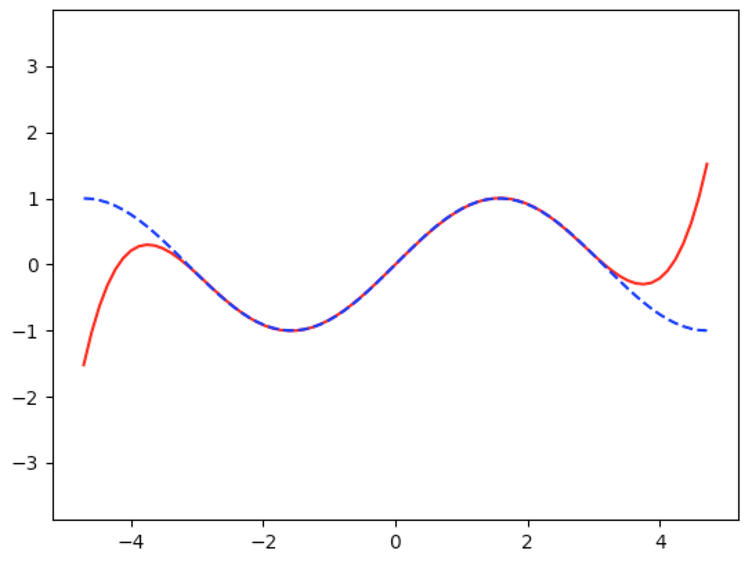
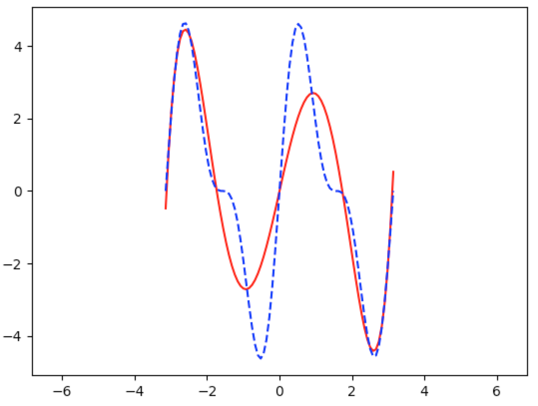
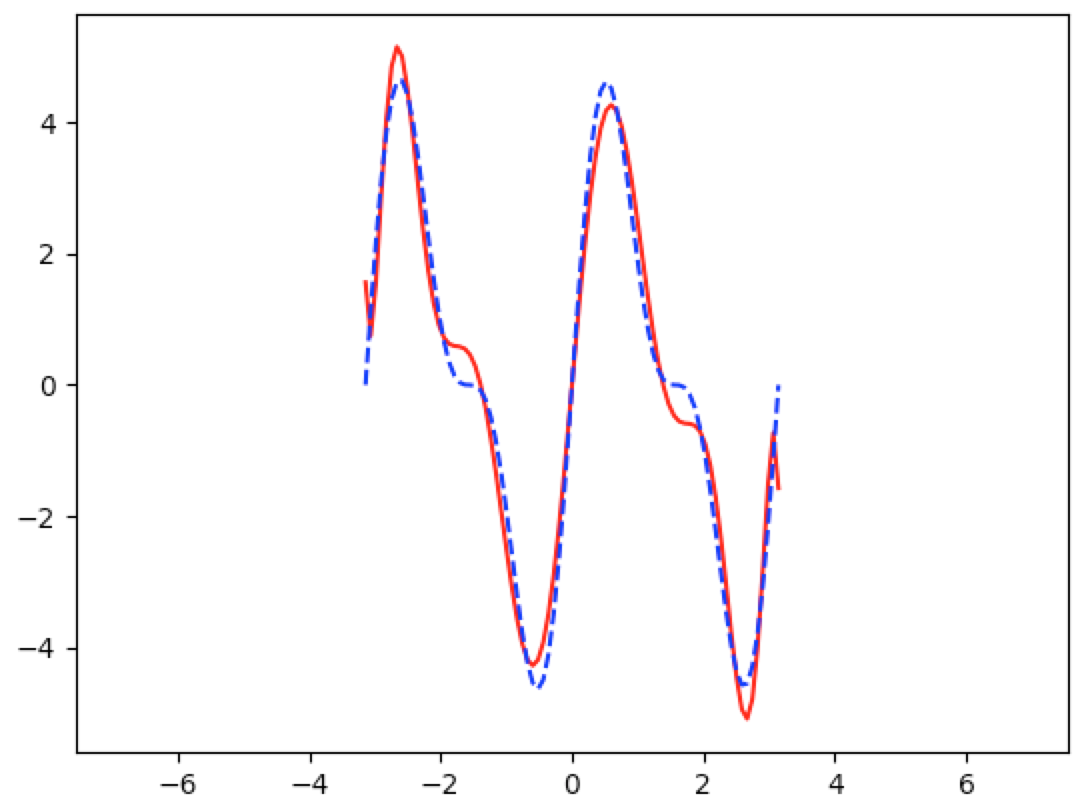
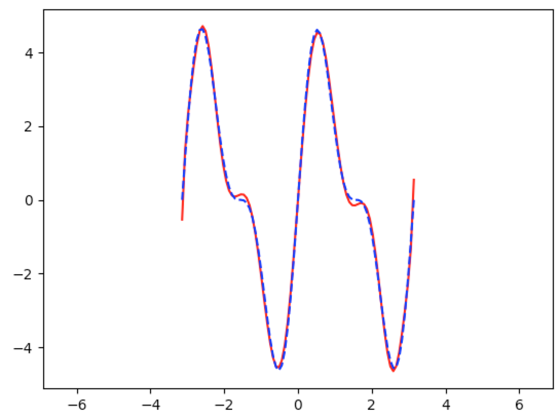
Let’s try this out on a more complicated function:
$$ v(t)\equiv15\cdot\sin{t}\cdot\cos^3{t}\cdot\exp{\Big(\frac1{t-19}\Big)} $$
Using a $5^{th}$ degree polynomial approximation, we get
And using an $11^{th}$ degree polynomial approximation, we get
And using a $13^{th}$ degree polynomial approximation, we get
Here is a more concrete but less flexible implementation of the same problem. It’s less flexible because we would have to make substantial changes to increase the degree of the approximation:
import numpy as np
import scipy.integrate as integrate
import matplotlib.pyplot as plt

I=lambda f_x,a,b: integrate.quad(f_x,a,b)[0]

func_mult=lambda f,g,t:f(t)*g(t)

func_innprd=lambda f,g: I(lambda t: func_mult(f,g,t),-np.pi,np.pi)

func_norm=lambda f: np.sqrt(func_innprd(f,f))

x0=lambda t: 1
x1=lambda t: t
x2=lambda t: t**2
x3=lambda t: t**3
x4=lambda t: t**4
x5=lambda t: t**5
x6=lambda t: t**6

nf0=func_norm(x0)
e0=lambda t: (1/nf0) * x0(t)

ip_x1e0=func_innprd(x1,e0)
ip_x2e0=func_innprd(x2,e0)
ip_x3e0=func_innprd(x3,e0)
ip_x4e0=func_innprd(x4,e0)
ip_x5e0=func_innprd(x5,e0)
print("ip_x1e0={}  ip_x2e0={}  ip_x3e0={}  ip_x4e0={}  ip_x5e0={}"
        .format(ip_x1e0,ip_x2e0,ip_x3e0,ip_x4e0,ip_x5e0))

f1=lambda w: x1(w)-ip_x1e0*e0(w)
nf1=func_norm(f1)
e1=lambda t: (1/nf1) * f1(t)

ip_x2e1=func_innprd(x2,e1)
ip_x3e1=func_innprd(x3,e1)
ip_x4e1=func_innprd(x4,e1)
ip_x5e1=func_innprd(x5,e1)
print("ip_x2e1={}  ip_x3e1={}  ip_x4e1={}  ip_x5e1={}".format(ip_x2e1,ip_x3e1,ip_x4e1,ip_x5e1))

f2=lambda w: x2(w)-(ip_x2e0 * e0(w) + ip_x2e1 * e1(w))
nf2=func_norm(f2)
e2=lambda t: (1/nf2) * f2(t)

ip_x3e2=func_innprd(x3,e2)
ip_x4e2=func_innprd(x4,e2)
ip_x5e2=func_innprd(x5,e2)
print("ip_x3e2={}  ip_x4e2={}  ip_x5e2={}".format(ip_x3e2,ip_x4e2,ip_x5e2))

f3=lambda w: x3(w)-(ip_x3e0 * e0(w) + ip_x3e1 * e1(w) + ip_x3e2 * e2(w))
nf3=func_norm(f3)
e3=lambda t: (1/nf3) * f3(t)

ip_x4e3=func_innprd(x4,e3)
ip_x5e3=func_innprd(x5,e3)
print("ip_x4e3={}  ip_x5e3={}".format(ip_x4e3,ip_x5e3))

f4=lambda w: x4(w)-(ip_x4e0 * e0(w) + ip_x4e1 * e1(w) + ip_x4e2 * e2(w) + ip_x4e3 * e3(w))
nf4=func_norm(f4)
e4=lambda t: (1/nf4) * f4(t)

ip_x5e4=func_innprd(x5,e4)
print("ip_x5e4={}".format(ip_x5e4))

f5=lambda w: x5(w)-(ip_x5e0 * e0(w) + ip_x5e1 * e1(w) + ip_x5e2 * e2(w) + ip_x5e3 * e3(w) + ip_x5e4 * e4(w))
nf5=func_norm(f5)
e5=lambda t: (1/nf5) * f5(t)

orthonormal_basis={0:e0,1:e1,2:e2,3:e3,4:e4,5:e5}

PUv=lambda v,t,n: np.sum(func_innprd(v,orthonormal_basis[i])*orthonormal_basis[i](t) for i in range(n))

def graph(funct, x_range, cl='r--', show=False):
    y_range=[]
    for x in x_range:
        y_range.append(funct(x))
    plt.plot(x_range,y_range,cl)
    return

rs=1.0
r=np.linspace(-rs*np.pi,rs*np.pi,100)
v=lambda t: 15*np.sin(t)*np.power(np.cos(t),3)*np.exp(1/(t-19))
v=np.sin
graph(lambda t: PUv(v,t,6),r,cl='r-')
graph(v,r,cl='b--')
plt.show()