Variance-Maximizing Dimension-Reduction
Suppose we are interviewing candidates for a software engineering role. And we suppose we have narrowed down our primary criteria to two variables: $x_{i,0}$ represents some measure of the software engineering enjoyment level of the $i^{th}$ candidate and $x_{i,1}$ represents some measure of the software engineering skill level of the $i^{th}$ candidate. Also suppose that we narrowed down the number of candidates to $20$. Using our measurements for these two variables, how can we select the best candidates?
First suppose that our measurements reveal that all $20$ candidates share the same skill level but have different enjoyment levels. Then skill level doesn’t differentiate one candidate from another. So we discard this variable and select the candidate with the highest enjoyment level. On the other hand, if all candidates share the same enjoyment level, then we choose the candidate with the highest skill level.
In either case above, the data is effectively reduced to a single dimension.
How do we select a candidate if they have different skill levels and different enjoyment levels? Suppose our measurements reveal that the candidate with the highest skill level has the lowest enjoyment level. It seems unlikely that that candidate would be as productive as some other candidates with lower skill levels but higher enjoyment levels. So what we really want to do is somehow reduce our two-dimensional data to a single variable that measures prospective productivity. Let’s construct some centered data:
import numpy as np
import matplotlib.pyplot as plt

covm=np.array([[1.7,3],[3,10]])

X=np.random.multivariate_normal([0,0],covm,size=(20,1)).reshape(20,2)

X=X-np.mean(X,axis=0)

np.mean(X,axis=0)
    array([  5.96744876e-17,  -6.66133815e-17])

np.set_printoptions(suppress=True)
np.round(X,3)
    array([[-1.27 , -4.109],
           [ 0.627,  4.411],
           [-1.125, -1.925],
           [ 1.744,  0.288],
           [ 1.341,  1.282],
           [-0.87 , -4.478],
           [-1.535, -3.009],
           [-0.005,  0.063],
           [ 0.945,  2.273],
           [-0.976, -2.912],
           [ 2.049,  4.164],
           [-0.533,  1.17 ],
           [-0.982, -3.964],
           [ 0.801,  2.977],
           [ 0.372, -0.443],
           [ 2.059,  3.826],
           [-2.574, -5.612],
           [-0.686,  1.624],
           [ 0.372,  2.775],
           [ 0.248,  1.599]])

plt.scatter(X[:,0],X[:,1])
    <matplotlib.collections.PathCollection at 0x1106f4b00>

lim=7;plt.xlim(-lim,lim);plt.ylim(-lim,lim)
    (-7, 7)

plt.gca().set_aspect('equal')

plt.show()
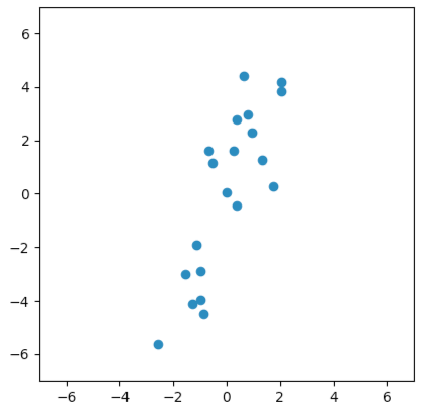
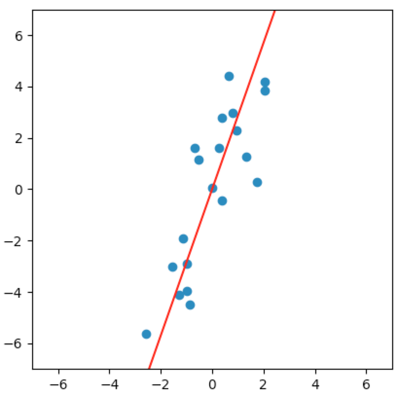
Just looking at the plot, we could reasonably conclude that there is almost a linear relationship between the two variables. We might say that the data could just as easily reside in some one-dimensional subspace of $\wR^2$. Said another way, it seems like we can orthogonally project the data onto some line going through the origin and not lose much information about the original data.
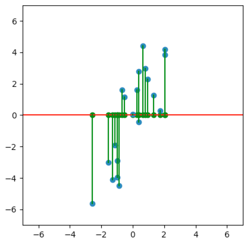
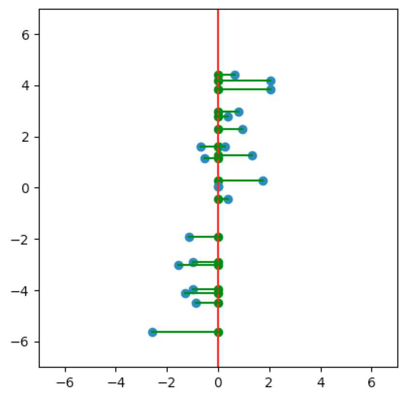
Let’s look at a few cases. In the first plot below, we project onto the span of the basis vector $(1,0)$. In the second plot, we project onto the span of the basis vector $(0,1)$. In the last plot, we project onto the span of some unknown basis vector. Note that the spread of the projections (green dots) varies by subspace (red line). Of the three, the second subspace has the largest spread while the third subspace has the smallest spread.
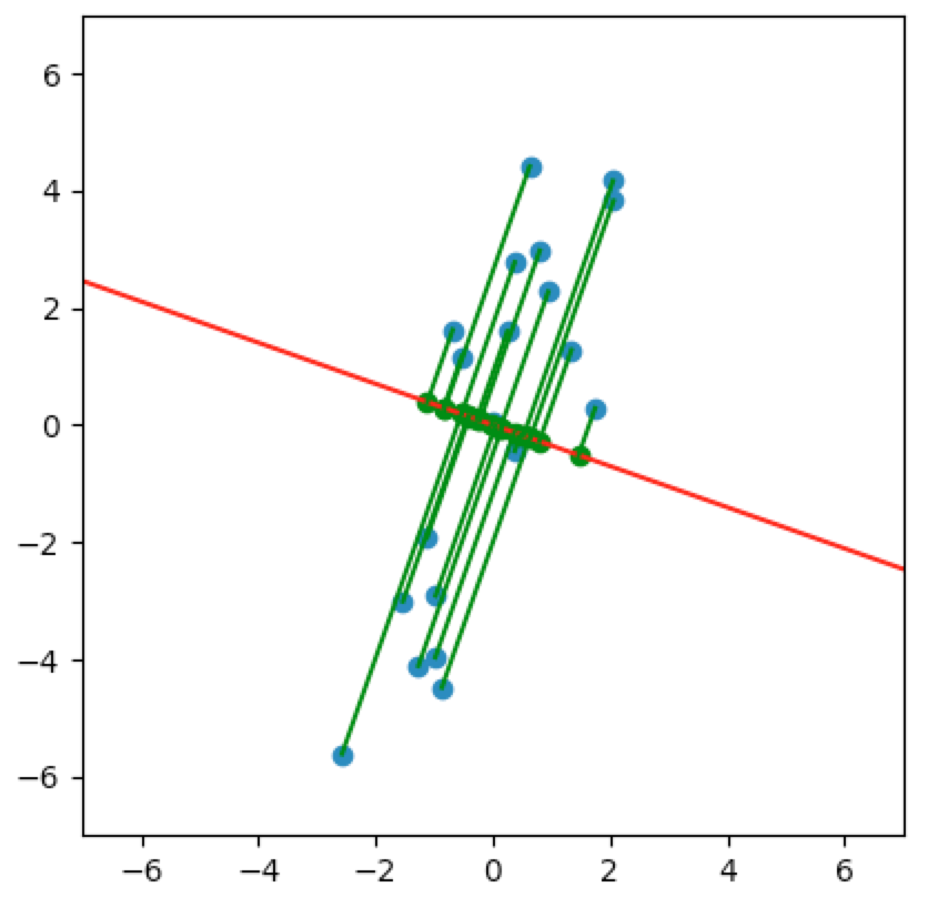
So how do we determine which is the best one-dimensional subspace to project onto? Since we want to select the best candidates, then we want our projection to retain data that captures the differences between candidates.
If one of the variables shows very little difference between candidates, then there’s less information to retain from this variable. If one of the variables shows large differences between candidates, then there’s more information to retain from this variable. So we want to retain more data from the variable with larger differences / variance. One way to try to maximize retention of variance / information / differences of the original data is to maximize the sample variance of the projection.
But we would also like to be able to reconstruct the original data from the projected data. To do this, we will make the basis vector of the one-dimensional subspace a linear combination of the basis in which the original data resides. Typically, the original basis is presumed to be the standard basis.
Hence our goal is to construct a basis (from the original basis) for the one-dimensional subspace that maximizes the sample variance of the projected data. Since an orthonormal basis provides a lot of helpful properties, we will also require that the vector in the new basis have unit length. We only require the angle of the one-dimensional subspace, so a unit length basis vector will suffice.
Let $e_1,e_2$ denote the standard basis of $\wR^2$ and let $x_i\in\wR^2$ denote the column vector representing the $i^{th}$ observation. Let $v\equiv ae_1+be_2$ be a linear combination of $e_1,e_2$ with unit length. Let $P_Ux$ denote the orthogonal projection of the vector $x$ onto the subspace $U$. Then Axler (6.55(i)) shows that
$$ P_{\span{v}}x_i=\innprd{x_i}{v}v $$
So our goal is to construct a unit length linear combination $v$ so as to maximize the (biased) sample variance of the orthogonal projections $P_{\span{v}}x_1,\dots,P_{\span{v}}x_{20}$. That is, we wish to compute
$$ \argmax{v:\dnorm{v}=1}\frac1{20}\sum_{i=1}^{20}\dnorm{\innprd{x_i}{v}v}^2 \tag{PCA.1} $$
Note that
$$ \dnorm{\innprd{x_i}{v}v}^2=\normw{\innprd{x_i}{v}}^2\dnorm{v}^2=\normw{\innprd{x_i}{v}}^2=\innprd{x_i}{v}^2=\innprd{x_i}{v}\innprd{x_i}{v}=\innprd{v}{x_i}\innprd{x_i}{v}=v^tx_ix_i^tv \tag{PCA.2} $$
and
$$ \frac1{20}\sum_{i=1}^{20}\dnorm{\innprd{x_i}{v}v}^2 = \frac1{20}\sum_{i=1}^{20}v^tx_ix_i^tv = v^t\prnfit{\frac1{20}\sum_{i=1}^{20}x_ix_i^t}v = v^tCv \tag{PCA.3} $$
where $C$ denotes the sample covariance matrix of the centered data $x_1,\dots,x_{20}$. Hence our constrainted maximization problem is
$$\align{ &\argmax{v:\dnorm{v}=1}v^tCv\\\\ }$$
We will use the method of Lagrangian multipliers to maximize this. The Lagrangian objective function becomes
$$ \lagrangsym(v,\lambda)=v^tCv-\lambda(v^tv-1) $$
The partial derivatives of $\lagrangsym$ are
$$ \nabla_v\lagrangsym(v,\lambda) = \nabla_v\prn{v^tCv-\lambda(v^tv-1)} = 2Cv-2\lambda v $$
and
$$ \wpart{\lagrangsym(v,\lambda)}{\lambda} = v^tv-1 $$
Setting the partial derivatives to zero, we get
$$ Cv=\lambda v\\ v^tv=1 $$
Hence a point $(v,\lambda)$ maximizes $\lagrangsym$ if and only if it’s an eigenpair of $C$ with $v$ having unit length and
$$ \lagrangsym(v,\lambda)=v^tCv-\lambda(v^tv-1)=v^tCv=v^t\lambda v=\lambda v^tv=\lambda $$
Since $\lagrangsym$ attains its maximum value at $v,\lambda$, we see that $\lambda$ is the maximum value of $\lagrangsym$. Now suppose $v’,\lambda’$ also maximizes $\lagrangsym$. Then $v’$ must be an eigenvector of $C$ (with unit length) corresponding to $\lambda’$. Performing the same computation as above tells us that $\lambda’$ and $\lambda$ are both equal to the global maximum value of the $\lagrangsym$. That is, $v$ and $v’$ share the same eigenvalue.
Said another way, a point maximizes $\lagrangsym$ if and only if it’s an eigenpair of $C$ consisting of the largest eigenvalue and a corresponding unit eigenvector. Hence a vector maximizes PCA.1 if and only if it’s a unit eigenvector of the sample covariance matrix corresponding to its largest eigenvalue. So let’s compute this eigenvector and the subspace it spans:
C=1/len(X)*X.T.dot(X)
C
    array([[ 1.54168804,  3.1267114 ],
           [ 3.1267114 ,  9.35168992]])

eigvals,eigvecs=np.linalg.eig(C)

eigvals
    array([  0.44415397,  10.44922399])
eigvecs
    array([[-0.94355827, -0.33120657],
           [ 0.33120657, -0.94355827]])

# We choose the second eigenvector because it
# corresponds to the largest eigenvalue 10.44922399.
v=eigvecs[:,1]
# For our purposes, the additive inverse -v of v
# will be more intuitive. Of course, -v is a unit
# eigenvector corresponding to 10.44922399. And
# span(v)=span(-v).
v=-v
v
    array([ 0.33120657,  0.94355827])

slope_of_subspace=v[1]/v[0]

xs=np.linspace(-lim,lim,100)

ys=xs*slope_of_subspace

plt.plot(xs,ys,'r')
    [<matplotlib.lines.Line2D at 0x11558c8d0>]

plt.scatter(X[:,0],X[:,1])
    <matplotlib.collections.PathCollection at 0x115594cc0>

plt.xlim(-lim,lim);plt.ylim(-lim,lim)
    (-7, 7)

plt.gca().set_aspect('equal')

plt.show()
And let’s project the data onto this subspace:
projections=[X[i].dot(v)*v for i in range(len(X))]

projections=np.array(projections)

plt.scatter(X[:,0],X[:,1])
    <matplotlib.collections.PathCollection at 0x121007ac8>

plt.plot(xs,ys,'r')
    [<matplotlib.lines.Line2D at 0x121007048>]

plt.scatter(projections[:,0],projections[:,1],c='g')
    <matplotlib.collections.PathCollection at 0x10c26cbe0>

for i in range(len(X)):
    plt.plot([X[i,0],projections[i,0]],[X[i,1],projections[i,1]],'g')

lim=7;plt.xlim(-lim,lim);plt.ylim(-lim,lim)
    (-7, 7)

plt.gca().set_aspect('equal')

plt.show()
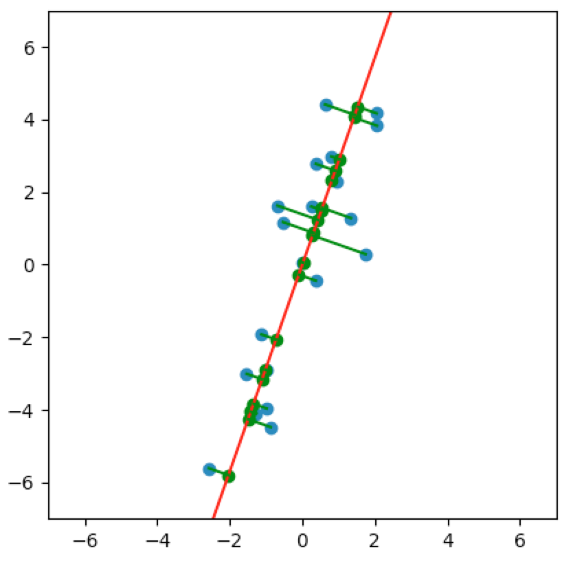
It’s not too difficult to see that the spread of the projections in the above subspace is larger than the spread of the projections in the subspaces we saw earlier:
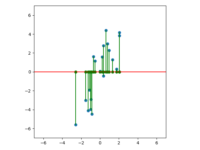
An animated view is helpful. Notice that the spread of green dots - the sample variance of our subspace projections - grows and shrinks depending on the subspace. And the spread attains its maximum at the subspace we identified above:
Recall that we want to project the original data onto this subspace to get a ranking of the prospective productivities of the candidates:
scores=X.dot(v)
np.round(scores,2)
   array([-4.3 ,  4.37, -2.19,  0.85,  1.65, -4.51, -3.35,  0.06,  2.46,
          -3.07,  4.61,  0.93, -4.07,  3.07, -0.3 ,  4.29, -6.15,  1.31,
           2.74,  1.59])

np.argsort(-scores)
    array([10,  1, 15, 13, 18,  8,  4, 19, 17, 11,  3,  7, 14,  2,  9,  6, 12,
            0,  5, 16])

np.round(np.hstack((X,scores.reshape(20,1)))[np.argsort(-scores)],2)
    array([[ 2.05,  4.16,  4.61],
           [ 0.63,  4.41,  4.37],
           [ 2.06,  3.83,  4.29],
           [ 0.8 ,  2.98,  3.07],
           [ 0.37,  2.77,  2.74],
           [ 0.94,  2.27,  2.46],
           [ 1.34,  1.28,  1.65],
           [ 0.25,  1.6 ,  1.59],
           [-0.69,  1.62,  1.31],
           [-0.53,  1.17,  0.93],
           [ 1.74,  0.29,  0.85],
           [-0.01,  0.06,  0.06],
           [ 0.37, -0.44, -0.3 ],
           [-1.12, -1.93, -2.19],
           [-0.98, -2.91, -3.07],
           [-1.54, -3.01, -3.35],
           [-0.98, -3.96, -4.07],
           [-1.27, -4.11, -4.3 ],
           [-0.87, -4.48, -4.51],
           [-2.57, -5.61, -6.15]])
So the $10^{th}$, $1^{st}$, and $15^{th}$ candidates (zero-index based) are our best choices with scores of $4.61$, $4.37$, and $4.29$, respectively. Now suppose that we have a new candidate for the software engineer role. And suppose we measure this new candidate’s enjoyment and skill levels at $1.57$ and $4.31$, respectively. Then we can compute this candidate’s prospective productivity score as well:
x_21=np.array([1.57,4.31])

x_21.dot(v)
    4.5867304563559985
Equivalence to Best Least-Squares Subspace
This process of variance-maximizing dimension-reduction is equivalent to finding the best least-squares subspace. Take another look at the plots above - both the animated and still plots. Note that the lengths of the green lines are shortest precisely when the variance is maximized, i.e., precisely when $v=(0.33, 0.94)$ is the eigenvector that we computed above.
We can make this statement precise. First note that
$$\align{ \dnorm{x_i-P_{\span{v}}x_i}^2 &= \dnorm{x_i-\innprd{x_i}{v}v}^2 \\ &= \innprdbg{x_i-\innprd{x_i}{v}v}{x_i-\innprd{x_i}{v}v} \\ &= \innprdbg{x_i}{x_i-\innprd{x_i}{v}v}+\innprdbg{-\innprd{x_i}{v}v}{x_i-\innprd{x_i}{v}v} \\ &= \innprd{x_i}{x_i}+\innprdbg{x_i}{-\innprd{x_i}{v}v}+\innprdbg{-\innprd{x_i}{v}v}{x_i}+\innprdbg{-\innprd{x_i}{v}v}{-\innprd{x_i}{v}v} \\ &= \innprd{x_i}{x_i}-\innprdbg{x_i}{\innprd{x_i}{v}v}-\innprdbg{\innprd{x_i}{v}v}{x_i}+\innprdbg{\innprd{x_i}{v}v}{\innprd{x_i}{v}v} \\ &= \innprd{x_i}{x_i}-\innprdbg{x_i}{\innprd{x_i}{v}v}-\innprdbg{x_i}{\innprd{x_i}{v}v}+\innprdbg{\innprd{x_i}{v}v}{\innprd{x_i}{v}v} \\ &= \dnorm{x_i}^2-2\innprdbg{x_i}{\innprd{x_i}{v}v}+\dnorm{\innprd{x_i}{v}v}^2 \\ &= \dnorm{x_i}^2-2\innprd{x_i}{v}\innprd{x_i}{v}+\dnorm{\innprd{x_i}{v}v}^2 \\ &= \dnorm{x_i}^2-2\norm{\innprd{x_i}{v}}^2+\dnorm{\innprd{x_i}{v}v}^2 \\ }$$
Hence
$$\align{ \argmin{v:\dnorm{v}=1}\sum_{i=1}^m\dnorm{x_i-P_{\span{v}}x_i}^2 &= \argmin{v:\dnorm{v}=1}\sum_{i=1}^m\prn{\dnorm{x_i}^2-2\norm{\innprd{x_i}{v}}^2+\dnorm{\innprd{x_i}{v}v}^2} \\ &= \argmin{v:\dnorm{v}=1}\sum_{i=1}^m\prn{-2\norm{\innprd{x_i}{v}}^2+\dnorm{\innprd{x_i}{v}v}^2}\tag{since $\dnorm{x_i}^2$ is constant wrt $v$} \\ &= \argmin{v:\dnorm{v}=1}\sum_{i=1}^m\prn{-2\norm{\innprd{x_i}{v}}^2\dnorm{v}^2+\dnorm{\innprd{x_i}{v}v}^2}\tag{since $\dnorm{v}^2=1$} \\ &= \argmin{v:\dnorm{v}=1}\sum_{i=1}^m\prn{-2\sbr{\norm{\innprd{x_i}{v}}\dnorm{v}}^2+\dnorm{\innprd{x_i}{v}v}^2} \\ &= \argmin{v:\dnorm{v}=1}\sum_{i=1}^m\prn{-2\dnorm{\innprd{x_i}{v}v}^2+\dnorm{\innprd{x_i}{v}v}^2} \\ &= \argmin{v:\dnorm{v}=1}\sum_{i=1}^m\prn{-\dnorm{\innprd{x_i}{v}v}^2} \\ &= \argmin{v:\dnorm{v}=1}\prnfit{-\sum_{i=1}^m\dnorm{\innprd{x_i}{v}v}^2} \\ &= \argmax{v:\dnorm{v}=1}\sum_{i=1}^{m}\dnorm{\innprd{x_i}{v}v}^2 \\ &= \argmax{v:\dnorm{v}=1}\sum_{i=1}^{m}\dnorm{P_{\span{v}}x_i}^2 }$$
Succinctly:
$$ \argmin{v:\dnorm{v}=1}\sum_{i=1}^m\dnorm{x_i-P_{\span{v}}x_i}^2 = \argmax{v:\dnorm{v}=1}\sum_{i=1}^{m}\dnorm{P_{\span{v}}x_i}^2 $$
Hence, we may synonymously say “variance-maximizing dimension-reduction”, “best least-squares subspace”, or “reconstruction error minimization”.
Connection with SVD
Note that the sample covariance matrix that we computed above is symmetric. More generally, suppose we have $m$ observations and $n$ variables. Then $X\in\wR^{m\times n}$ and
$$ C^t=\Prn{\frac1mX^tX}^t=\frac1m(X^tX)^t=\frac1mX^t(X^t)^t=\frac1mX^tX=C $$
Hence, by the Spectral Theorem, $C$ is diagonalizable. That is, there exists an orthonormal basis $v_{:,1},\dots,v_{:,n}$ of $\wR^n$ that consists of eigenvectors of $C$ and we get the diagonalization (or Spectral Decomposition)
$$ C=V\Lambda V^t =\pmtrx{v_{1,1}&\dotsb&v_{1,n}\\\vdots&\ddots&\vdots\\v_{n,1}&\dotsb&v_{n,n}} \pmtrx{\frac{\lambda_1}{m}&\dotsb&0\\\vdots&\ddots&\vdots\\0&\dotsb&\frac{\lambda_n}{m}} \pmtrx{v_{1,1}&\dotsb&v_{1,n}\\\vdots&\ddots&\vdots\\v_{n,1}&\dotsb&v_{n,n}}^t \tag{CWS.1} $$
$\Lambda$ is diagonal with the eigenvalues of $C$ on its diagonal. $V$ consists of the column vectors $v_{:,1},\dots,v_{:,n}$. The eigenvector $v_{:,j}$ corresponds the eigenvalue $\frac{\lambda_j}{m}$. Axler 7.24 and 7.29 cover diagonalization from the Spectral Theorem, although he omits coverage of the Spectral Decomposition, which is just a change of basis. In my post Polar Decomposition & SVD, I extend Axler’s coverage to include the change of basis (SPECT.1).
From PCA.2 and PCA.3, we can see that, for any $v\in\wR^n$, we have
$$ v^tCv = \frac1{m}\sum_{i=1}^{m}\norm{\innprd{x_i}{v}}^2 \geq 0 $$
Hence $C$ is positive semi-definite. Hence $\lambda_j$ must be nonnegative (by App.28 and Axler 7.35(b)). Also note that
$$ X^tXv_{:,j}=\frac{m}{m}X^tXv_{:,j}=m\Prn{\frac1{m}X^tX}v_{:,j}=mCv_{:,j}=m\frac{\lambda_j}{m}v_{:,j}=\lambda_jv_{:,j} \tag{CWS.2} $$
Hence $\lambda_j$ is an eigenvalue of $X^tX$ corresponding to the eigenvector $v_{:,j}$. Then the Singular Value Decomposition of $X$ is
$$ X=USV^t =\pmtrx{u_{1,1}&\dotsb&u_{1,n}\\\vdots&\ddots&\vdots\\\vdots&\ddots&\vdots\\u_{m,1}&\dotsb&u_{m,n}} \pmtrx{\sqrt{\lambda_1}&\dotsb&0\\\vdots&\ddots&\vdots\\0&\dotsb&\sqrt{\lambda_n}} \pmtrx{v_{1,1}&\dotsb&v_{1,n}\\\vdots&\ddots&\vdots\\v_{n,1}&\dotsb&v_{n,n}}^t \tag{CWS.3} $$
where $V$ still consists of the column vectors $v_{:,1},\dots,v_{:,n}$ (by SVD.1.E). $S$ is diagonal with the singular values of $X$ on the diagonal. The singular values are equal to the square roots of the eigenvalues of $X^tX$ (by SVD.1.D). Since the columns of $V$ are orthonormal, then App.26 gives $V^tV=I_n$ and
$$ XV=US $$
and
$$ Xv_{:,1}=\pmtrx{\innprd{x_1}{v_{:,1}}\\\vdots\\\innprd{x_m}{v_{:,1}}} =\pmtrx{\innprd{x_1}{v_{:,1}}&\dotsb&\innprd{x_1}{v_{:,n}}\\\vdots&\ddots&\vdots\\\innprd{x_m}{v_{:,1}}&\dotsb&\innprd{x_m}{v_{:,n}}}_{:,1}=(XV)_{:,1} =(US)_{:,1} =\pmtrx{u_{1,1}\sqrt{\lambda_1}\\\vdots\\u_{m,1}\sqrt{\lambda_1}} =\sqrt{\lambda_1}u_{:,1} $$
We will assume that the singular values on the diagonal of $S$ and the eigenvalues on the diagonal of $\Lambda$ are ordered from largest to smallest (re-index if necessary). So if we want to compute the best one-dimensional subspace and corresponding scores as we did in the example, we can compute the SVD of $X$:
U,S,VT=np.linalg.svd(X,full_matrices=False)

U.shape,S.shape,VT.shape
    ((20, 2), (2,), (2, 2))

S
    array([ 14.45629551,   2.98044954])

S[0]**2/len(X)
    10.449223991840675

# note that the above computation gives the largest eigenvalue of C
eigvals
    array([  0.44415397,  10.44922399])

# said another way:
np.sqrt(len(X)*eigvals[1])
    14.456295508767576

VT.T
    array([[-0.33120657, -0.94355827],
           [-0.94355827,  0.33120657]])

# Hence v=-V[:,0] and the optimal 1-dimensional subspace is span(-V[:,0])
# Hence we will use the SVD (-U)np.diag(S)(-VT). Hence

np.round(S[0]*-U[:,0],2)
    array([-4.3 ,  4.37, -2.19,  0.85,  1.65, -4.51, -3.35,  0.06,  2.46,
           -3.07,  4.61,  0.93, -4.07,  3.07, -0.3 ,  4.29, -6.15,  1.31,
            2.74,  1.59])

np.round(scores,2)
    array([-4.3 ,  4.37, -2.19,  0.85,  1.65, -4.51, -3.35,  0.06,  2.46,
           -3.07,  4.61,  0.93, -4.07,  3.07, -0.3 ,  4.29, -6.15,  1.31,
            2.74,  1.59])
There is a more efficient computation of the basis vector of the best one-dimensional subspace that is often used. Since the number of observations $m$ is generally much larger than the number of variables $n$, then the covariance matrix $C_{n\times n}$ is much smaller than the data matrix $X_{m\times n}$. If the covariance matrix $C$ is invertible, then SVD.4 shows that an SVD of the covariance matrix is also a Spectral Decomposition.
In our example, the covariance matrix is invertible:
np.linalg.inv(C)
    array([[ 2.0149882 , -0.67370568],
           [-0.67370568,  0.33218415]])
Hence
cU,cS,cVT=np.linalg.svd(C,full_matrices=True)

cU.shape,cS.shape,cVT.shape
    ((2, 2), (2,), (2, 2))

cU
    array([[-0.33120657, -0.94355827],
           [-0.94355827,  0.33120657]])

cS
    array([ 10.44922399,   0.44415397])

cVT
    array([[-0.33120657, -0.94355827],
           [-0.94355827,  0.33120657]])

np.round(X.dot(-cU[:,0]),2)
    array([-4.3 ,  4.37, -2.19,  0.85,  1.65, -4.51, -3.35,  0.06,  2.46,
           -3.07,  4.61,  0.93, -4.07,  3.07, -0.3 ,  4.29, -6.15,  1.31,
            2.74,  1.59])

np.round(scores,2)
    array([-4.3 ,  4.37, -2.19,  0.85,  1.65, -4.51, -3.35,  0.06,  2.46,
           -3.07,  4.61,  0.93, -4.07,  3.07, -0.3 ,  4.29, -6.15,  1.31,
            2.74,  1.59])
Terminology
We’ve seen the benefits of reducing to a one-dimensional subspace. But we will soon see that reduction to a multi-dimensional subspace is also very helpful, very intuitive, and widely performed. And we will find that the first $k$ column vectors in the matrix $V$ of either SVD (CWS.3) or Spectral Decomposition (CWS.1) gives an othornormal basis of the best $k$-dimensional subspace.
Suppose we have performed PCA to compute the best $k$-dimensional subspace. Then the vectors in the eigenbasis of that best subspace are called principal axes or principal components. That is, the column vectors of $V$ from CWS.3 or CWS.1 are the principal components or principal axes. The columns of $US=XV$ are called the PC scores or just the scores. Sometimes the scores are also called the principal components.
Data Standardization
It’s generally more convenient to work with centered data. That is, we subtract the variable means from each observed value. That is, we first compute the means of the observed data for each variable:
$$ \mu\equiv\frac1m\sum_{i=1}^mx_i \dq\iff\dq \mu_j\equiv\frac1m\sum_{i=1}^mx_{i,j}\qd\text{for }j=1,\dots,n $$
And then we reset the observed data:
$$ x_i=x_i-\mu \dq\iff\dq x_{i,j}=x_{i,j}-\mu_j\qd\text{for }j=1,\dots,n $$
In our constructed example, we computed:
X=X-np.mean(X,axis=0)
We do so to simplify the computation of the sample covariance matrix:
C=1/len(X)*X.T.dot(X)
C
    array([[ 1.54168804,  3.1267114 ],
           [ 3.1267114 ,  9.35168992]])
If the data is not centered, we can still compute the sample covariance matrix. For instance, suppose in our example that the means of the first and second variables are $3$ and $6$, respectively. Then the uncentered data is
uX=np.hstack(((X[:,0]+3).reshape(20,1),(X[:,1]+6).reshape(20,1)))
uX
    array([[  1.72954251,   1.89116317],
           [  3.62683021,  10.41092788],
           [  1.87546335,   4.07487126],
           [  4.74412361,   6.28810546],
           [  4.34054259,   7.28161875],
           [  2.12965288,   1.52183383],
           [  1.46495154,   2.99056588],
           [  2.99450253,   6.06333105],
           [  3.94476976,   8.2730544 ],
           [  2.02421263,   3.08796258],
           [  5.04945924,  10.16438551],
           [  2.46676862,   7.16999132],
           [  2.01795813,   2.03624394],
           [  3.80073967,   8.97694348],
           [  3.37217416,   5.55662994],
           [  5.05910605,   9.82594254],
           [  0.42592579,   0.38849958],
           [  2.31401708,   7.62394889],
           [  3.37170589,   8.77475398],
           [  3.24755374,   7.59922655]])
Then we can compute the sample covariance matrix:
uC=1/len(uX)*(uX-np.mean(uX,axis=0)).T.dot((uX-np.mean(uX,axis=0)))
uC
    array([[ 1.54168804,  3.1267114 ],
           [ 3.1267114 ,  9.35168992]])
This sample covariance matrix agrees with the above computation but is less convenient to compute.
Additionally, in equations CWS.1, CWS.2, and CWS.3, we showed the connections between PCA and SVD. But we used the equality $C=\frac1mX^tX$ in CWS.2. Hence CWS.2 and CWS.3 only hold if $X$ has been centered. Hence this pre-processing step of centering the data must be done if we use the SVD of $X$ for PCA purposes.
In addition to centering the data, we should also consider the scale of each variable. By scale, we refer to two things: the unit of measure for each variable and the variance of each variable.
First suppose that the unit of measure is different. For example, suppose we want to rank the value of houses in a given neighborhood. And suppose we consider two variables: the number of bedrooms and the square footage:
uhX=np.array([[3,1450],[4,2450],[2,2100],[4,2800],[3,2250],[5,3400],[6,2750],[2,1050],[3,2550],[2,1650]])
uhX
    array([[   3, 1450],
           [   4, 2450],
           [   2, 2100],
           [   4, 2800],
           [   3, 2250],
           [   5, 3400],
           [   6, 2750],
           [   2, 1050],
           [   3, 2550],
           [   2, 1650]])
So we center the data, compute the eigendecomposition of its sample covariance matrix, and compute the scores:
hX=uhX-np.mean(uhX,axis=0)
hX
    array([[   -0.4,  -795. ],
           [    0.6,   205. ],
           [   -1.4,  -145. ],
           [    0.6,   555. ],
           [   -0.4,     5. ],
           [    1.6,  1155. ],
           [    2.6,   505. ],
           [   -1.4, -1195. ],
           [   -0.4,   305. ],
           [   -1.4,  -595. ]])

hC=1/len(hX)*hX.T.dot(hX)
hC
    array([[      1.64,     652.  ],
           [    652.  ,  446725.  ]])

h_eigvals,h_eigvecs=np.linalg.eig(hC)
h_eigvals
    array([      0.68839744,  446725.95160256])

h_eigvecs
    array([[-0.99999893, -0.00145951],
           [ 0.00145951, -0.99999893]])

h_v=-h_eigvecs[:,1]

h_scores=hX.dot(h_v)

np.hstack((uhX,h_scores.reshape(10,1)))[np.argsort(-h_scores)]
    array([[    5.        ,  3400.        ,  1155.00110504],
           [    4.        ,  2800.        ,   555.00028458],
           [    6.        ,  2750.        ,   505.00325686],
           [    3.        ,  2550.        ,   304.99909134],
           [    4.        ,  2450.        ,   205.00065736],
           [    3.        ,  2250.        ,     4.99941087],
           [    2.        ,  2100.        ,  -145.00188888],
           [    2.        ,  1650.        ,  -595.00140959],
           [    3.        ,  1450.        ,  -794.99973706],
           [    2.        ,  1050.        , -1195.00077054]])
Notice that the ranking gives almost zero weight to the first variable, the number of bedrooms. We can see this in the first principal component:
h_v
    array([ 0.00145951,  0.99999893])
The first variable is almost completely disregarded. This is reflected in the ranking.
There is a commonly used approach to balance the weights for each variable. We divide the observations for each variable by that variable’s standard deviation:
h_0_sd=np.sqrt(hC[0,0])
h_1_sd=np.sqrt(hC[1,1])

whX=np.hstack(((hX[:,0]/h_0_sd).reshape(10,1),(hX[:,1]/h_1_sd).reshape(10,1)))
whX
    array([[-0.31234752, -1.18945222],
           [ 0.46852129,  0.30671409],
           [-1.09321633, -0.21694411],
           [ 0.46852129,  0.8303723 ],
           [-0.31234752,  0.00748083],
           [ 1.2493901 ,  1.72807209],
           [ 2.0302589 ,  0.75556399],
           [-1.09321633, -1.78791874],
           [-0.31234752,  0.45633072],
           [-1.09321633, -0.89021895]])

# Note that the norms of each variable are equal:
np.linalg.norm(whX[:,0]),np.linalg.norm(whX[:,1]),np.sqrt(10)
    (3.1622776601683786, 3.16227766016838, 3.1622776601683795)

whC=1/len(whX)*whX.T.dot(whX)
whC
    array([[ 1.        ,  0.76173786],
           [ 0.76173786,  1.        ]])

# Note that this is just the sample correlation matrix of hX:
hC[0,1]/(h_0_sd*h_1_sd)
    0.76173786256376796

wh_eigvals,wh_eigvecs=np.linalg.eig(whC)
wh_eigvals
    array([ 0.23826214,  1.76173786])

wh_eigvecs
    array([[-0.70710678, -0.70710678],
           [ 0.70710678, -0.70710678]])

wh_v=-wh_eigvecs[:,1]
wh_v
    array([ 0.70710678,  0.70710678])

wh_scores=whX.dot(wh_v)

np.hstack((uhX,wh_scores.reshape(10,1)))[np.argsort(-wh_scores)]
    array([[    5.        ,  3400.        ,     2.1053837 ],
           [    6.        ,  2750.        ,     1.96987426],
           [    4.        ,  2800.        ,     0.91845646],
           [    4.        ,  2450.        ,     0.54817419],
           [    3.        ,  2550.        ,     0.1018115 ],
           [    3.        ,  2250.        ,    -0.21557331],
           [    2.        ,  2100.        ,    -0.92642334],
           [    3.        ,  1450.        ,    -1.06193278],
           [    2.        ,  1650.        ,    -1.40250054],
           [    2.        ,  1050.        ,    -2.03727015]])

np.hstack((uhX,h_scores.reshape(10,1)))[np.argsort(-h_scores)]
    array([[    5.        ,  3400.        ,  1155.00110504],
           [    4.        ,  2800.        ,   555.00028458],
           [    6.        ,  2750.        ,   505.00325686],
           [    3.        ,  2550.        ,   304.99909134],
           [    4.        ,  2450.        ,   205.00065736],
           [    3.        ,  2250.        ,     4.99941087],
           [    2.        ,  2100.        ,  -145.00188888],
           [    2.        ,  1650.        ,  -595.00140959],
           [    3.        ,  1450.        ,  -794.99973706],
           [    2.        ,  1050.        , -1195.00077054]])
Now we want to consider the case where the unit of measure is the same for the variables but the variance is different. Returning to our example of selecting the best software engineer candidates, suppose the data that we constructed uses the same unit of measure for enjoyment and skill levels. For concreteness, suppose that, for the uncentered data, both variables are measured on a scale from $0$ to $12$. Also suppose that the mean of the uncentered data for each variable is $6$. Then
uX=np.hstack(((X[:,0]+6).reshape(20,1),(X[:,1]+6).reshape(20,1)))
uX
    array([[  4.72954251,   1.89116317],
           [  6.62683021,  10.41092788],
           [  4.87546335,   4.07487126],
           [  7.74412361,   6.28810546],
           [  7.34054259,   7.28161875],
           [  5.12965288,   1.52183383],
           [  4.46495154,   2.99056588],
           [  5.99450253,   6.06333105],
           [  6.94476976,   8.2730544 ],
           [  5.02421263,   3.08796258],
           [  8.04945924,  10.16438551],
           [  5.46676862,   7.16999132],
           [  5.01795813,   2.03624394],
           [  6.80073967,   8.97694348],
           [  6.37217416,   5.55662994],
           [  8.05910605,   9.82594254],
           [  3.42592579,   0.38849958],
           [  5.31401708,   7.62394889],
           [  6.37170589,   8.77475398],
           [  6.24755374,   7.59922655]])
It’s helpful to see the above data. But when we center it, we of course just get the original centered data matrix $X$:
wX=uX-np.mean(uX,axis=0)
wX-X
    array([[ 0.,  0.],
           [ 0.,  0.],
           [ 0.,  0.],
           [ 0.,  0.],
           [ 0.,  0.],
           [ 0.,  0.],
           [ 0.,  0.],
           [ 0.,  0.],
           [ 0.,  0.],
           [ 0.,  0.],
           [ 0.,  0.],
           [ 0.,  0.],
           [ 0.,  0.],
           [ 0.,  0.],
           [ 0.,  0.],
           [ 0.,  0.],
           [ 0.,  0.],
           [ 0.,  0.],
           [ 0.,  0.],
           [ 0.,  0.]])

C=1/len(X)*X.T.dot(X)
C
  array([[ 1.54168804,  3.1267114 ],
         [ 3.1267114 ,  9.35168992]])
Note that the sample variances differ between the two variables. The second is substantially larger than the first. As a result, the linear combination used to compute the score (i.e., the principal component) gives a bigger weight to the second variable:
eigvals,eigvecs=np.linalg.eig(C)
eigvals
    array([  0.44415397,  10.44922399])

eigvecs
    array([[-0.94355827, -0.33120657],
           [ 0.33120657, -0.94355827]])

v
    array([ 0.33120657,  0.94355827])
In this case, this principal component seems appropriate. The enjoyment and skill levels are measured in the same units. But the variance of the skill level is much greater than that of the enjoyment level. That is, our measurements of skill level show much greater differences between candidates than do our measurements of enjoyment level. And we want our one-dimensional subspace and the corresponding rankings to reflect that.
Deeper Perspective
Suppose a single observation consists of $n$ real-valued variables. Then an observation is a vector in $\wR^n$, which has the standard basis $e\equiv e_1,\dots,e_n$. Equivalently, we can think of the observed value of the $j^{th}$ variable as a vector in $\span{e_j}$ so that an observation of all $n$ variables is a vector in $\bigoplus_{j=1}^n\span{e_j}=\span{e_1,\dots,e_n}=\wR^n$.
Said another way, the sample space is $\wR^n$ and the outcome of a single random experiment is a vector in $\wR^n$.
Now suppose we’re given an $m\times n$ matrix $X$ consisting of $m$ observations of these $n$ variables. Let $g\equiv g_1,\dots,g_{m}$ be the standard basis of $\wR^{m}$ and define $T\in\linmap{\wR^n}{\wR^{m}}$ by
$$ Te_1\equiv\sum_{i=1}^{m}X_{i,1}g_i \dq\dotsb\dq Te_n\equiv\sum_{i=1}^{m}X_{i,n}g_i $$
Hence, by Axler 3.32, we have
$$ X=\pmtrx{X_{1,1}&\dotsb&X_{1,n}\\\vdots&\ddots&\vdots\\\vdots&\ddots&\vdots\\X_{m,1}&\dotsb&X_{m,n}} =\mtrxof{T,e,g} $$
Hence, we can regard the linear map $T$ as the execution of a set of random experiments from the sample space $\wR^n$ to the outcome or observation space $\wR^{m}$.
Note that SVD.1.A gives
$$\align{ \mtrxof{T,e,g} &= \mtrxof{S,f,g}\mtrxofb{\sqrttat,f}\mtrxof{I,f,e}^t \\ &= \pmtrx{\innprd{Sf_1}{g_1}&\dotsb&\innprd{Sf_n}{g_1}\\\vdots&\ddots&\vdots\\\vdots&\ddots&\vdots\\\innprd{Sf_1}{g_m}&\dotsb&\innprd{Sf_n}{g_m}} \pmtrx{\sqrt{\lambda_1}&\dots&0\\\vdots&\ddots&\vdots\\0&\dots&\sqrt{\lambda_n}} \pmtrx{\innprd{f_1}{e_1}&\dotsb&\innprd{f_n}{e_1}\\\vdots&\ddots&\vdots\\\innprd{f_1}{e_n}&\dotsb&\innprd{f_n}{e_n}}^t \\ }$$
where $f\equiv f_1,\dots,f_n$ is an orthonormal basis of $\wR^n$ that consists of eigenvectors of $\tat$ corresponding to the eigenvalues $\lambda_1,\dots,\lambda_n$ and where
$$ Sf_j=\cases{\frac1{\sqrt{\lambda_j}}Tf_j&\text{for }j=1,\dots,\dim{\rangsp{T}}\\h_j&\text{for }j=\dim{\rangsp{T}}+1,\dots,n} $$
where $h_{\dim{\rangsp{T}}+1},\dots,h_n$ is any orthonormal list in $\rangsp{T}^\perp$ of length $n-\dim{\rangsp{T}}$. If $\dim{\rangsp{T}}=n$, then the rank of $X=\mtrxof{T,e,g}$ is $n$ (by Axler 3.117, 3.118, and 3.119). Hence the columns of $X$ are linearly independent. The same argument works in reverse as well. Hence, if the variables are linearly independent, then
$$ Sf_j=\frac1{\sqrt{\lambda_j}}Tf_j\qd\text{for }j=1,\dots,n \tag{DP.1} $$
If the columns of $X$ are not linearly independent, then we have a redundant variable that we remove. Hence we always assume that the columns of $X$ are linearly independent and, hence, that DP.1 holds.
Note that, for $j=1,\dots,n$, we have
$$ Tf_j=T\prnfit{\sum_{p=1}^{n}\innprd{f_j}{e_p}e_p}=\sum_{p=1}^{n}\innprd{f_j}{e_p}Te_p=\sum_{p=1}^{n}\innprd{f_j}{e_p}\sum_{i=1}^{m}X_{i,p}g_i $$
Hence, for $k=1,\dots,m$, we have
$$\align{ \innprd{Tf_j}{g_k} &= \innprdBgg{\sum_{p=1}^{n}\innprd{f_j}{e_p}\sum_{i=1}^{m}X_{i,p}g_i}{g_k} = \sum_{p=1}^{n}\innprd{f_j}{e_p}\sum_{i=1}^{m}X_{i,p}\innprd{g_i}{g_k} = \sum_{p=1}^{n}\innprd{f_j}{e_p}X_{k,p} \\ &= \sum_{p=1}^{n}\innprd{f_j}{e_p}\innprd{X_k}{e_p} = \sum_{p=1}^{n}\innprdbg{X_k}{\innprd{f_j}{e_p}e_p} = \innprdBgg{X_k}{\sum_{p=1}^{n}\innprd{f_j}{e_p}e_p} = \innprd{X_k}{f_j} }$$
and
$$ \innprd{Sf_j}{g_k}=\innprdBg{\frac1{\sqrt{\lambda_j}}Tf_j}{g_k}=\frac1{\sqrt{\lambda_j}}\innprd{Tf_j}{g_k}=\frac1{\sqrt{\lambda_j}}\innprd{X_k}{f_j} $$
and our scores matrix is
$$\align{ \mtrxof{S,f,g}\mtrxofb{\sqrttat,f} &= \pmtrx{\innprd{Sf_1}{g_1}&\dotsb&\innprd{Sf_n}{g_1}\\\vdots&\ddots&\vdots\\\vdots&\ddots&\vdots\\\innprd{Sf_1}{g_m}&\dotsb&\innprd{Sf_n}{g_m}} \pmtrx{\sqrt{\lambda_1}&\dots&0\\\vdots&\ddots&\vdots\\0&\dots&\sqrt{\lambda_n}} \\\\ &= \pmtrx{\sqrt{\lambda_1}\innprd{Sf_1}{g_1}&\dotsb&\sqrt{\lambda_n}\innprd{Sf_n}{g_1}\\\vdots&\ddots&\vdots\\\vdots&\ddots&\vdots\\\sqrt{\lambda_1}\innprd{Sf_1}{g_m}&\dotsb&\sqrt{\lambda_n}\innprd{Sf_n}{g_m}} \\\\ &= \pmtrx{\sqrt{\lambda_1}\frac1{\sqrt{\lambda_1}}\innprd{X_1}{f_1}&\dotsb&\sqrt{\lambda_n}\frac1{\sqrt{\lambda_n}}\innprd{X_1}{f_n}\\\vdots&\ddots&\vdots\\\vdots&\ddots&\vdots\\\sqrt{\lambda_1}\frac1{\sqrt{\lambda_1}}\innprd{X_m}{f_1}&\dotsb&\sqrt{\lambda_n}\frac1{\sqrt{\lambda_n}}\innprd{X_m}{f_n}} \\\\ &= \pmtrx{\innprd{X_1}{f_1}&\dotsb&\innprd{X_1}{f_n}\\\vdots&\ddots&\vdots\\\vdots&\ddots&\vdots\\\innprd{X_m}{f_1}&\dotsb&\innprd{X_m}{f_n}} \tag{DP.2} }$$
Scores
Now we will show that the scores vector produces a meaningful ranking. Recall that the first principal axis $f_1$ is chosen to maximize the sample variance. That is,
$$ f_1\equiv\argmax{f\in\wR^n:\dnorm{f}=1}\sum_{i=1}^m\dnorm{\innprd{X_i}{f}f}^2=\argmax{f\in\wR^n:\dnorm{f}=1}\sum_{i=1}^m\innprd{X_i}{f}^2 $$
The second equality holds because, if $\dnorm{f}=1$, then
$$ \dnorm{\innprd{X_i}{f}f}^2=\prn{\normw{\innprd{X_i}{f}}\dnorm{f}}^2=\norm{\innprd{X_i}{f}}^2=\innprd{X_i}{f}^2 $$
By Axler 6.30 and 6.55(i), $\span{f_1}$ is the one-dimensional subspace that maximizes the sum of the projections of $X_1,\dots,X_m$. Since $\span{f_1}$ is one-dimensional, then it’s isomorphic to $\wR$ (by Axler 3.59). Hence we can think of $\span{f_1}$ as $\wR$.
Note that App.1 shows that there are exactly two unit basis vectors of $\span{f_1}$. They are $f_1$ and $-f_1$. So which one should we use?
Recall from our earlier example that we found an eigenvector $v$ of the covariance matrix $C$ and then we flipped the sign. Then we computed the scores:
scores=X.dot(v)
np.round(np.hstack((X,scores.reshape(20,1)))[np.argsort(-scores)],2)
    array([[ 2.05,  4.16,  4.61],
           [ 0.63,  4.41,  4.37],
           [ 2.06,  3.83,  4.29],
           [ 0.8 ,  2.98,  3.07],
           [ 0.37,  2.77,  2.74],
           [ 0.94,  2.27,  2.46],
           [ 1.34,  1.28,  1.65],
           [ 0.25,  1.6 ,  1.59],
           [-0.69,  1.62,  1.31],
           [-0.53,  1.17,  0.93],
           [ 1.74,  0.29,  0.85],
           [-0.01,  0.06,  0.06],
           [ 0.37, -0.44, -0.3 ],
           [-1.12, -1.93, -2.19],
           [-0.98, -2.91, -3.07],
           [-1.54, -3.01, -3.35],
           [-0.98, -3.96, -4.07],
           [-1.27, -4.11, -4.3 ],
           [-0.87, -4.48, -4.51],
           [-2.57, -5.61, -6.15]])
But we could have used the eigenvector that we originally computed:
neg_scores=X.dot(-v)
np.round(np.hstack((X,neg_scores.reshape(20,1)))[np.argsort(-neg_scores)],2)
    array([[-2.57, -5.61,  6.15],
           [-0.87, -4.48,  4.51],
           [-1.27, -4.11,  4.3 ],
           [-0.98, -3.96,  4.07],
           [-1.54, -3.01,  3.35],
           [-0.98, -2.91,  3.07],
           [-1.12, -1.93,  2.19],
           [ 0.37, -0.44,  0.3 ],
           [-0.01,  0.06, -0.06],
           [ 1.74,  0.29, -0.85],
           [-0.53,  1.17, -0.93],
           [-0.69,  1.62, -1.31],
           [ 0.25,  1.6 , -1.59],
           [ 1.34,  1.28, -1.65],
           [ 0.94,  2.27, -2.46],
           [ 0.37,  2.77, -2.74],
           [ 0.8 ,  2.98, -3.07],
           [ 2.06,  3.83, -4.29],
           [ 0.63,  4.41, -4.37],
           [ 2.05,  4.16, -4.61]])
Clearly $\span{v}=\span{-v}$. But notice that the ranking for $-v$ is the opposite of the ranking for $v$. In particular, notice that the ranking for $v$ ranks “positive vectors” higher and “negative vectors” lower. And the ranking for $-v$ does the opposite.
By “positive vectors”, we mean those vectors with more positive components than negative components. In this example, and in most cases, we want to rank positive vectors higher. Note that a score is a linear combination (or weighted average) of the components of the observation:
\[\innprd{X_i}{f_1}=\innprdBgg{X_i}{\sum_{j=1}^n\innprd{f_1}{e_j}e_j}=\sum_{j=1}^n\innprdbg{X_i}{\innprd{f_1}{e_j}e_j}=\sum_{j=1}^n\innprd{f_1}{e_j}\innprd{X_i}{e_j}=\sum_{j=1}^n\innprd{f_1}{e_j}X_{i,j}\]So how do we systematically know which of $f_1$ or $-f_1$ ranks the positive vectors higher? The most direct approach is to test the whether the observation with the highest score is positive. Alternatively, we can compute $\innprd{f_1}{\sum_{j=1}^ne_n}$ to test whether $f_1$ is positive.
Reduction to Multi-Dimensional Subspaces
Note that SVD.1.G gives
$$ \mtrxof{T,e,g} = \sum_{j=1}^{\dim{\rangsp{T}}}\sqrt{\lambda_j}\mtrxof{Sf_j,g}\adjt{\mtrxof{f_j,e}} \tag{RMDS.1} $$
Also note that each term in the sum is a rank one matrix. Hence we can compute a rank $k$ matrix approximation to $X=\mtrxof{T,e,g}$ for $k=1,\dots,n$:
$$ \mtrxof{T,e,g} \approx \sum_{j=1}^{k}\sqrt{\lambda_j}\mtrxof{Sf_j,g}\adjt{\mtrxof{f_j,e}} \tag{RMDS.2} $$
We can also iteratively compute the maximum sample variance of the orthogonal projections:
$$ f_1\equiv\argmax{f\in\wR^n:\dnorm{f}=1}\sum_{i=1}^m\dnorm{\innprd{X_i}{f}f}^2 $$
$$ f_2\equiv\argmax{f\perp f_1:\dnorm{f}=1}\sum_{i=1}^m\dnorm{\innprd{X_i}{f}f}^2 $$
$$ \vdots $$
$$ f_n\equiv\argmax{f\perp f_1,\dots,f_{n-1}:\dnorm{f}=1}\sum_{i=1}^m\dnorm{\innprd{X_i}{f}f}^2 $$
Earlier we used Lagrangian multipliers to show that the solution to the first argmax problem gives an eigenpair of the covariance matrix $C$. We can also show that each of the successive argmax solutions gives an eigenpair of $C$. By CWS.2, each eigenpair $\frac{\lambda_j}{m},f_j$ of $C$ corresponds to the singular value $\sqrt{\lambda_j}$ and right singular vector $f_j$ of $X=\mtrxof{T,e,g}$. Hence the solutions to these argmax problems also give the rank $k$ matrix approximations to $X=\mtrxof{T,e,g}$. Lastly, we can also show that these approximations are best-fit or optimal.
Recommender System
Suppose we run a movie recommendation app/website. If a user has already watched a movie, then that user can rate it. Suppose the ratings are from $1$ to $5$, with $1$ being the worst rating and $5$ being the best possible rating. Also suppose we have $5$ movies in our database: Matrix, Star Wars, Alien, Titanic, and Casablanca. Also suppose that we have $20$ users who have already watched and rated these $5$ movies. Let’s construct some data:
covm=np.full((5,5),3.)
covm
    array([[ 3.,  3.,  3.,  3.,  3.],
           [ 3.,  3.,  3.,  3.,  3.],
           [ 3.,  3.,  3.,  3.,  3.],
           [ 3.,  3.,  3.,  3.,  3.],
           [ 3.,  3.,  3.,  3.,  3.]])

covm[3,0:3]=-2.7
covm[4,0:3]=-2.7
covm[0:3,3]=-2.7
covm[0:3,4]=-2.7
covm
    array([[ 3. ,  3. ,  3. , -2.7, -2.7],
           [ 3. ,  3. ,  3. , -2.7, -2.7],
           [ 3. ,  3. ,  3. , -2.7, -2.7],
           [-2.7, -2.7, -2.7,  3. ,  3. ],
           [-2.7, -2.7, -2.7,  3. ,  3. ]])

for i in range(5):
    for j in range(5):
        if i==j or covm[i,j]<0: continue
        covm[i,j]=2.7

covm
    array([[ 3. ,  2.7,  2.7, -2.7, -2.7],
           [ 2.7,  3. ,  2.7, -2.7, -2.7],
           [ 2.7,  2.7,  3. , -2.7, -2.7],
           [-2.7, -2.7, -2.7,  3. ,  2.7],
           [-2.7, -2.7, -2.7,  2.7,  3. ]])

Xo=np.random.multivariate_normal([3,3,3,3,3],covm,size=(20,1)).reshape(20,5)
np.round(Xo,0)
    array([[ 1.,  2.,  1.,  4.,  5.],
           [ 5.,  5.,  4.,  2.,  1.],
           [ 3.,  2.,  2.,  4.,  5.],
           [ 3.,  4.,  3.,  3.,  2.],
           [ 2.,  2.,  2.,  4.,  3.],
           [ 4.,  4.,  5.,  2.,  2.],
           [ 2.,  2.,  1.,  4.,  4.],
           [ 5.,  5.,  5.,  1.,  1.],
           [ 4.,  4.,  5.,  2.,  2.],
           [ 4.,  3.,  4.,  2.,  1.],
           [ 3.,  3.,  2.,  5.,  3.],
           [-0.,  0., -0.,  6.,  6.],
           [ 3.,  3.,  3.,  3.,  4.],
           [ 4.,  3.,  3.,  1.,  2.],
           [ 0.,  1.,  0.,  5.,  5.],
           [ 6.,  7.,  6.,  0., -0.],
           [ 3.,  2.,  3.,  4.,  3.],
           [ 4.,  5.,  4.,  1.,  2.],
           [ 1.,  1.,  1.,  6.,  4.],
           [ 3.,  4.,  4.,  1.,  3.]])

Xo=np.array(Xo,dtype=int)
Xo=np.maximum(Xo,1)
Xo=np.minimum(Xo,5)
Xo
    array([[1, 1, 1, 3, 4],
           [4, 4, 3, 2, 1],
           [2, 1, 1, 4, 4],
           [3, 4, 2, 2, 2],
           [2, 1, 1, 4, 3],
           [3, 3, 4, 1, 1],
           [1, 1, 1, 4, 3],
           [5, 5, 5, 1, 1],
           [4, 4, 4, 1, 1],
           [3, 3, 4, 1, 1],
           [2, 3, 1, 4, 3],
           [1, 1, 1, 5, 5],
           [2, 3, 2, 3, 3],
           [3, 3, 2, 1, 1],
           [1, 1, 1, 5, 4],
           [5, 5, 5, 1, 1],
           [3, 2, 2, 3, 3],
           [4, 4, 4, 1, 1],
           [1, 1, 1, 5, 4],
           [3, 3, 3, 1, 2]])

xoU,xoS,xoVT=np.linalg.svd(Xo,full_matrices=False)

np.round(xoS,2)
    array([ 25.75,  12.86,   2.47,   1.72,   1.53])

np.round([np.sum(xoS[:i])/np.sum(xoS) for i in range(1,6)],2)
    array([ 0.58,  0.87,  0.93,  0.97,  1.  ])

X=Xo-np.mean(Xo,axis=0)
X
    array([[-1.65, -1.65, -1.4 ,  0.4 ,  1.6 ],
           [ 1.35,  1.35,  0.6 , -0.6 , -1.4 ],
           [-0.65, -1.65, -1.4 ,  1.4 ,  1.6 ],
           [ 0.35,  1.35, -0.4 , -0.6 , -0.4 ],
           [-0.65, -1.65, -1.4 ,  1.4 ,  0.6 ],
           [ 0.35,  0.35,  1.6 , -1.6 , -1.4 ],
           [-1.65, -1.65, -1.4 ,  1.4 ,  0.6 ],
           [ 2.35,  2.35,  2.6 , -1.6 , -1.4 ],
           [ 1.35,  1.35,  1.6 , -1.6 , -1.4 ],
           [ 0.35,  0.35,  1.6 , -1.6 , -1.4 ],
           [-0.65,  0.35, -1.4 ,  1.4 ,  0.6 ],
           [-1.65, -1.65, -1.4 ,  2.4 ,  2.6 ],
           [-0.65,  0.35, -0.4 ,  0.4 ,  0.6 ],
           [ 0.35,  0.35, -0.4 , -1.6 , -1.4 ],
           [-1.65, -1.65, -1.4 ,  2.4 ,  1.6 ],
           [ 2.35,  2.35,  2.6 , -1.6 , -1.4 ],
           [ 0.35, -0.65, -0.4 ,  0.4 ,  0.6 ],
           [ 1.35,  1.35,  1.6 , -1.6 , -1.4 ],
           [-1.65, -1.65, -1.4 ,  2.4 ,  1.6 ],
           [ 0.35,  0.35,  0.6 , -1.6 , -0.4 ]])

np.mean(X,axis=0)
    array([  8.88178420e-17,   8.88178420e-17,   8.88178420e-17,
            -8.88178420e-17,   8.88178420e-17])

np.set_printoptions(suppress=True)

C=1/len(X)*X.T.dot(X)
C
    array([[ 1.6275,  1.6275,  1.64  , -1.64  , -1.46  ],
           [ 1.6275,  1.9275,  1.69  , -1.74  , -1.56  ],
           [ 1.64  ,  1.69  ,  2.04  , -1.89  , -1.61  ],
           [-1.64  , -1.74  , -1.89  ,  2.34  ,  1.86  ],
           [-1.46  , -1.56  , -1.61  ,  1.86  ,  1.74  ]])

xU,xS,xVT=np.linalg.svd(X,full_matrices=False)
xU.shape,xS.shape,xVT.shape
    ((20, 5), (5,), (5, 5))

np.round(xS,2)
    array([ 13.16,   3.07,   2.41,   1.7 ,   1.52])

np.round([np.sum(xS[:i])/np.sum(xS) for i in range(1,6)],2)
    array([ 0.6 ,  0.74,  0.85,  0.93,  1.  ])

f1=xVT[0]
f2=xVT[1]

vo=np.array([1,1,1,1,1])
f1.dot(vo)
    0.39567321966761149

np.round(f1,2)
array([ 0.41,  0.44,  0.46, -0.49, -0.43])

np.round(f2,2)
array([-0.39, -0.54, -0.14, -0.65, -0.34])

m_scores=X.dot(f1)
m_scores2=X.dot(f2)

np.round(np.hstack((Xo,m_scores.reshape(20,1)))[np.argsort(-m_scores)],2)
    array([[ 5.  ,  5.  ,  5.  ,  1.  ,  1.  ,  4.59],
           [ 5.  ,  5.  ,  5.  ,  1.  ,  1.  ,  4.59],
           [ 4.  ,  4.  ,  4.  ,  1.  ,  1.  ,  3.27],
           [ 4.  ,  4.  ,  4.  ,  1.  ,  1.  ,  3.27],
           [ 3.  ,  3.  ,  4.  ,  1.  ,  1.  ,  2.42],
           [ 3.  ,  3.  ,  4.  ,  1.  ,  1.  ,  2.42],
           [ 4.  ,  4.  ,  3.  ,  2.  ,  1.  ,  2.32],
           [ 3.  ,  3.  ,  3.  ,  1.  ,  2.  ,  1.53],
           [ 3.  ,  3.  ,  2.  ,  1.  ,  1.  ,  1.5 ],
           [ 3.  ,  4.  ,  2.  ,  2.  ,  2.  ,  1.02],
           [ 2.  ,  3.  ,  2.  ,  3.  ,  3.  , -0.75],
           [ 3.  ,  2.  ,  2.  ,  3.  ,  3.  , -0.78],
           [ 2.  ,  3.  ,  1.  ,  4.  ,  3.  , -1.7 ],
           [ 2.  ,  1.  ,  1.  ,  4.  ,  3.  , -2.58],
           [ 1.  ,  1.  ,  1.  ,  3.  ,  4.  , -2.93],
           [ 1.  ,  1.  ,  1.  ,  4.  ,  3.  , -3.  ],
           [ 2.  ,  1.  ,  1.  ,  4.  ,  4.  , -3.01],
           [ 1.  ,  1.  ,  1.  ,  5.  ,  4.  , -3.92],
           [ 1.  ,  1.  ,  1.  ,  5.  ,  4.  , -3.92],
           [ 1.  ,  1.  ,  1.  ,  5.  ,  5.  , -4.34]])

np.round(np.hstack((Xo,m_scores2.reshape(20,1)))[np.argsort(-m_scores2)],2)
    array([[ 3.  ,  3.  ,  2.  ,  1.  ,  1.  ,  1.24],
           [ 3.  ,  3.  ,  4.  ,  1.  ,  1.  ,  0.97],
           [ 3.  ,  3.  ,  4.  ,  1.  ,  1.  ,  0.97],
           [ 1.  ,  1.  ,  1.  ,  3.  ,  4.  ,  0.93],
           [ 3.  ,  3.  ,  3.  ,  1.  ,  2.  ,  0.76],
           [ 1.  ,  1.  ,  1.  ,  4.  ,  3.  ,  0.62],
           [ 2.  ,  1.  ,  1.  ,  4.  ,  3.  ,  0.23],
           [ 4.  ,  4.  ,  4.  ,  1.  ,  1.  ,  0.03],
           [ 4.  ,  4.  ,  4.  ,  1.  ,  1.  ,  0.03],
           [ 2.  ,  1.  ,  1.  ,  4.  ,  4.  , -0.11],
           [ 3.  ,  2.  ,  2.  ,  3.  ,  3.  , -0.19],
           [ 3.  ,  4.  ,  2.  ,  2.  ,  2.  , -0.29],
           [ 2.  ,  3.  ,  2.  ,  3.  ,  3.  , -0.34],
           [ 1.  ,  1.  ,  1.  ,  5.  ,  4.  , -0.37],
           [ 1.  ,  1.  ,  1.  ,  5.  ,  4.  , -0.37],
           [ 4.  ,  4.  ,  3.  ,  2.  ,  1.  , -0.48],
           [ 1.  ,  1.  ,  1.  ,  5.  ,  5.  , -0.71],
           [ 2.  ,  3.  ,  1.  ,  4.  ,  3.  , -0.85],
           [ 5.  ,  5.  ,  5.  ,  1.  ,  1.  , -1.04],
           [ 5.  ,  5.  ,  5.  ,  1.  ,  1.  , -1.04]])
Notice that the ranking in the first subspace is meaningful while the ranking in the second subspace is not. It is also helpful to see this with the centered data:
np.round(np.hstack((X,m_scores.reshape(20,1)))[np.argsort(-m_scores)],2)
    array([[ 2.35,  2.35,  2.6 , -1.6 , -1.4 ,  4.59],
           [ 2.35,  2.35,  2.6 , -1.6 , -1.4 ,  4.59],
           [ 1.35,  1.35,  1.6 , -1.6 , -1.4 ,  3.27],
           [ 1.35,  1.35,  1.6 , -1.6 , -1.4 ,  3.27],
           [ 0.35,  0.35,  1.6 , -1.6 , -1.4 ,  2.42],
           [ 0.35,  0.35,  1.6 , -1.6 , -1.4 ,  2.42],
           [ 1.35,  1.35,  0.6 , -0.6 , -1.4 ,  2.32],
           [ 0.35,  0.35,  0.6 , -1.6 , -0.4 ,  1.53],
           [ 0.35,  0.35, -0.4 , -1.6 , -1.4 ,  1.5 ],
           [ 0.35,  1.35, -0.4 , -0.6 , -0.4 ,  1.02],
           [-0.65,  0.35, -0.4 ,  0.4 ,  0.6 , -0.75],
           [ 0.35, -0.65, -0.4 ,  0.4 ,  0.6 , -0.78],
           [-0.65,  0.35, -1.4 ,  1.4 ,  0.6 , -1.7 ],
           [-0.65, -1.65, -1.4 ,  1.4 ,  0.6 , -2.58],
           [-1.65, -1.65, -1.4 ,  0.4 ,  1.6 , -2.93],
           [-1.65, -1.65, -1.4 ,  1.4 ,  0.6 , -3.  ],
           [-0.65, -1.65, -1.4 ,  1.4 ,  1.6 , -3.01],
           [-1.65, -1.65, -1.4 ,  2.4 ,  1.6 , -3.92],
           [-1.65, -1.65, -1.4 ,  2.4 ,  1.6 , -3.92],
           [-1.65, -1.65, -1.4 ,  2.4 ,  2.6 , -4.34]])

np.round(np.hstack((X,m_scores2.reshape(20,1)))[np.argsort(-m_scores2)],2)
    array([[ 0.35,  0.35, -0.4 , -1.6 , -1.4 ,  1.24],
           [ 0.35,  0.35,  1.6 , -1.6 , -1.4 ,  0.97],
           [ 0.35,  0.35,  1.6 , -1.6 , -1.4 ,  0.97],
           [-1.65, -1.65, -1.4 ,  0.4 ,  1.6 ,  0.93],
           [ 0.35,  0.35,  0.6 , -1.6 , -0.4 ,  0.76],
           [-1.65, -1.65, -1.4 ,  1.4 ,  0.6 ,  0.62],
           [-0.65, -1.65, -1.4 ,  1.4 ,  0.6 ,  0.23],
           [ 1.35,  1.35,  1.6 , -1.6 , -1.4 ,  0.03],
           [ 1.35,  1.35,  1.6 , -1.6 , -1.4 ,  0.03],
           [-0.65, -1.65, -1.4 ,  1.4 ,  1.6 , -0.11],
           [ 0.35, -0.65, -0.4 ,  0.4 ,  0.6 , -0.19],
           [ 0.35,  1.35, -0.4 , -0.6 , -0.4 , -0.29],
           [-0.65,  0.35, -0.4 ,  0.4 ,  0.6 , -0.34],
           [-1.65, -1.65, -1.4 ,  2.4 ,  1.6 , -0.37],
           [-1.65, -1.65, -1.4 ,  2.4 ,  1.6 , -0.37],
           [ 1.35,  1.35,  0.6 , -0.6 , -1.4 , -0.48],
           [-1.65, -1.65, -1.4 ,  2.4 ,  2.6 , -0.71],
           [-0.65,  0.35, -1.4 ,  1.4 ,  0.6 , -0.85],
           [ 2.35,  2.35,  2.6 , -1.6 , -1.4 , -1.04],
           [ 2.35,  2.35,  2.6 , -1.6 , -1.4 , -1.04]])
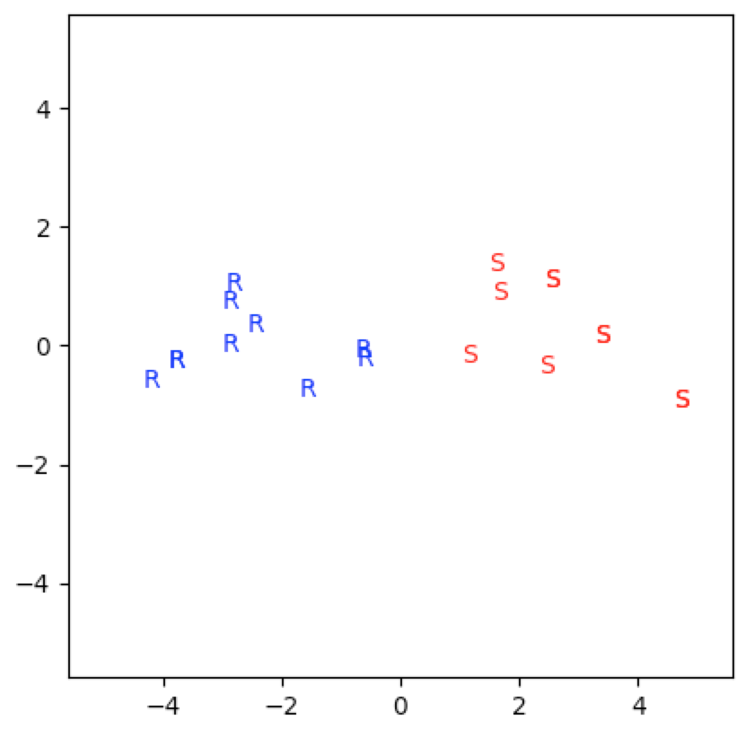
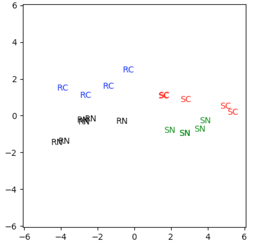
So what’s going on here? Why is the first subspace ranking significant while the second subspace ranking insignificant? The reason is that SVD captures in the first subspace the two genres of film and the film covariances. And this is really the bulk of the meaningful information from this dataset.
We can see this from the first singular value and the first principal component. The first subspace captures $60\%$ of the information and the first principal component captures the covariances between the movies. The positivity of the first three components and the negativity of the last two components of $f_1$ capture the two genres sci-fi and romance. And $f_2$ only captures $14\%$ of the information from the dataset:
np.round(xS,2)
    array([ 13.16,   3.07,   2.41,   1.7 ,   1.52])

np.round([np.sum(xS[:i])/np.sum(xS) for i in range(1,6)],2)
    array([ 0.6 ,  0.74,  0.85,  0.93,  1.  ])

f1=xVT[0]
f2=xVT[1]

np.round(f1,2)
array([ 0.41,  0.44,  0.46, -0.49, -0.43])

np.round(f2,2)
array([-0.39, -0.54, -0.14, -0.65, -0.34])
We can also see this geometrically:
genre=[1 if np.mean(X[i,:3])>=np.mean(X[i,3:5]) else 2 for i in range(20)]

genre
    [2, 1, 2, 1, 2, 1, 2, 1, 1, 1, 2, 2, 2, 1, 2, 1, 2, 1, 2, 1]

xt=20*['S']

xtc=20*['red']

for i in range(20):
    if genre[i]==1: xt[i],xtc[i]='S','red'
    if genre[i]==2: xt[i],xtc[i]='R','blue'

xt=np.array(xt)
xtc=np.array(xtc)

np.hstack((Xo,xt.reshape(20,1),xtc.reshape(20,1)))
    array([['1', '1', '1', '3', '4', 'R', 'blue'],
           ['4', '4', '3', '2', '1', 'S', 'red'],
           ['2', '1', '1', '4', '4', 'R', 'blue'],
           ['3', '4', '2', '2', '2', 'S', 'red'],
           ['2', '1', '1', '4', '3', 'R', 'blue'],
           ['3', '3', '4', '1', '1', 'S', 'red'],
           ['1', '1', '1', '4', '3', 'R', 'blue'],
           ['5', '5', '5', '1', '1', 'S', 'red'],
           ['4', '4', '4', '1', '1', 'S', 'red'],
           ['3', '3', '4', '1', '1', 'S', 'red'],
           ['2', '3', '1', '4', '3', 'R', 'blue'],
           ['1', '1', '1', '5', '5', 'R', 'blue'],
           ['2', '3', '2', '3', '3', 'R', 'blue'],
           ['3', '3', '2', '1', '1', 'S', 'red'],
           ['1', '1', '1', '5', '4', 'R', 'blue'],
           ['5', '5', '5', '1', '1', 'S', 'red'],
           ['3', '2', '2', '3', '3', 'R', 'blue'],
           ['4', '4', '4', '1', '1', 'S', 'red'],
           ['1', '1', '1', '5', '4', 'R', 'blue'],
           ['3', '3', '3', '1', '2', 'S', 'red']],
          dtype='<U21')

fcs=[{'color':xtc[i]} for i in range(20)]

for i in range(len(m_scores)):
    plt.text(m_scores[i],m_scores2[i],xt[i],fontdict=fcs[i])

pe=np.max(np.abs(np.stack((m_scores,m_scores2))))+1

plt.xlim((-pe,pe))
    (-5.5858411049768835, 5.5858411049768835)

plt.ylim((-pe,pe))
    (-5.5858411049768835, 5.5858411049768835)

plt.gca().set_aspect('equal')

plt.show()
Now suppose that a couple of new users come along. Each of these new users has only watched one of the movies from our current list and we want to recommend a movie:
x_21=np.mean(X,axis=0)

x_21
array([ 0.,  0.,  0., -0.,  0.])

x_21[3]=np.max(X[:,3])

x_21
array([ 0. ,  0. ,  0. ,  2.4,  0. ])

x_21.dot(f1)
-1.1806768206805012

# Hence user x_21 would probably enjoy a romance

x_22=np.mean(X,axis=0)

x_22
array([ 0.,  0.,  0., -0.,  0.])

x_22[1]=np.max(X[:,1])

x_22
array([ 0.  ,  2.35,  0.  , -0.  ,  0.  ])

x_22.dot(f1)
1.0373307995880079

# Hence user x_22 would probably enjoy a sci-fi
Now let’s append a couple movies to our variable space. We’ll append the crime films Scarface and Godfather:
Xe=np.array([[2,3],[4,3],[2,3],[4,3],[2,3],[3,2],[3,4],[4,3],[3,2],[3,2],[3,4],[1,2],[4,5],[3,4],[1,2],[5,2],[2,3],[4,2],[2,5],[3,2]])

Xe
    array([[2, 3],
           [4, 3],
           [2, 3],
           [4, 3],
           [2, 3],
           [3, 2],
           [3, 4],
           [4, 3],
           [3, 2],
           [3, 2],
           [3, 4],
           [1, 2],
           [4, 5],
           [3, 4],
           [1, 2],
           [5, 2],
           [2, 3],
           [4, 2],
           [2, 5],
           [3, 2]])

Xes=np.hstack((Xo,Xe))
Xes
    array([[1, 1, 1, 3, 4, 2, 3],
           [4, 4, 3, 2, 1, 4, 3],
           [2, 1, 1, 4, 4, 2, 3],
           [3, 4, 2, 2, 2, 4, 3],
           [2, 1, 1, 4, 3, 2, 3],
           [3, 3, 4, 1, 1, 3, 2],
           [1, 1, 1, 4, 3, 3, 4],
           [5, 5, 5, 1, 1, 4, 3],
           [4, 4, 4, 1, 1, 3, 2],
           [3, 3, 4, 1, 1, 3, 2],
           [2, 3, 1, 4, 3, 3, 4],
           [1, 1, 1, 5, 5, 1, 2],
           [2, 3, 2, 3, 3, 4, 5],
           [3, 3, 2, 1, 1, 3, 4],
           [1, 1, 1, 5, 4, 1, 2],
           [5, 5, 5, 1, 1, 5, 2],
           [3, 2, 2, 3, 3, 2, 3],
           [4, 4, 4, 1, 1, 4, 2],
           [1, 1, 1, 5, 4, 2, 5],
           [3, 3, 3, 1, 2, 3, 2]])

eX=Xes-np.mean(Xes,axis=0)
eX
    array([[-1.65, -1.65, -1.4 ,  0.4 ,  1.6 , -0.9 ,  0.05],
           [ 1.35,  1.35,  0.6 , -0.6 , -1.4 ,  1.1 ,  0.05],
           [-0.65, -1.65, -1.4 ,  1.4 ,  1.6 , -0.9 ,  0.05],
           [ 0.35,  1.35, -0.4 , -0.6 , -0.4 ,  1.1 ,  0.05],
           [-0.65, -1.65, -1.4 ,  1.4 ,  0.6 , -0.9 ,  0.05],
           [ 0.35,  0.35,  1.6 , -1.6 , -1.4 ,  0.1 , -0.95],
           [-1.65, -1.65, -1.4 ,  1.4 ,  0.6 ,  0.1 ,  1.05],
           [ 2.35,  2.35,  2.6 , -1.6 , -1.4 ,  1.1 ,  0.05],
           [ 1.35,  1.35,  1.6 , -1.6 , -1.4 ,  0.1 , -0.95],
           [ 0.35,  0.35,  1.6 , -1.6 , -1.4 ,  0.1 , -0.95],
           [-0.65,  0.35, -1.4 ,  1.4 ,  0.6 ,  0.1 ,  1.05],
           [-1.65, -1.65, -1.4 ,  2.4 ,  2.6 , -1.9 , -0.95],
           [-0.65,  0.35, -0.4 ,  0.4 ,  0.6 ,  1.1 ,  2.05],
           [ 0.35,  0.35, -0.4 , -1.6 , -1.4 ,  0.1 ,  1.05],
           [-1.65, -1.65, -1.4 ,  2.4 ,  1.6 , -1.9 , -0.95],
           [ 2.35,  2.35,  2.6 , -1.6 , -1.4 ,  2.1 , -0.95],
           [ 0.35, -0.65, -0.4 ,  0.4 ,  0.6 , -0.9 ,  0.05],
           [ 1.35,  1.35,  1.6 , -1.6 , -1.4 ,  1.1 , -0.95],
           [-1.65, -1.65, -1.4 ,  2.4 ,  1.6 , -0.9 ,  2.05],
           [ 0.35,  0.35,  0.6 , -1.6 , -0.4 ,  0.1 , -0.95]])


exU,exS,exVT=np.linalg.svd(eX,full_matrices=False)
np.round(exS,2)
    array([ 13.79,   4.77,   3.09,   1.98,   1.86,   1.6 ,   1.31])

np.round([np.sum(exS[:i])/np.sum(exS) for i in range(1,8)],2)
    array([ 0.49,  0.65,  0.76,  0.83,  0.9 ,  0.95,  1.  ])

ef1=exVT[0]
ef2=exVT[1]

np.round(ef1,2)
    array([ 0.39,  0.42,  0.44, -0.47, -0.41,  0.28, -0.12])

np.round(ef2,2)
    array([-0.01,  0.25, -0.24,  0.12, -0.06,  0.46,  0.81])

e_scores=eX.dot(ef1)
e_scores2=eX.dot(ef2)

np.round(np.hstack((Xes,e_scores.reshape(20,1)))[np.argsort(-e_scores)],2)
    array([[ 5.  ,  5.  ,  5.  ,  1.  ,  1.  ,  5.  ,  2.  ,  5.07],
           [ 5.  ,  5.  ,  5.  ,  1.  ,  1.  ,  4.  ,  3.  ,  4.67],
           [ 4.  ,  4.  ,  4.  ,  1.  ,  1.  ,  4.  ,  2.  ,  3.54],
           [ 4.  ,  4.  ,  4.  ,  1.  ,  1.  ,  3.  ,  2.  ,  3.26],
           [ 4.  ,  4.  ,  3.  ,  2.  ,  1.  ,  4.  ,  3.  ,  2.51],
           [ 3.  ,  3.  ,  4.  ,  1.  ,  1.  ,  3.  ,  2.  ,  2.44],
           [ 3.  ,  3.  ,  4.  ,  1.  ,  1.  ,  3.  ,  2.  ,  2.44],
           [ 3.  ,  3.  ,  3.  ,  1.  ,  2.  ,  3.  ,  2.  ,  1.6 ],
           [ 3.  ,  3.  ,  2.  ,  1.  ,  1.  ,  3.  ,  4.  ,  1.33],
           [ 3.  ,  4.  ,  2.  ,  2.  ,  2.  ,  4.  ,  3.  ,  1.28],
           [ 2.  ,  3.  ,  2.  ,  3.  ,  3.  ,  4.  ,  5.  , -0.65],
           [ 3.  ,  2.  ,  2.  ,  3.  ,  3.  ,  2.  ,  3.  , -1.  ],
           [ 2.  ,  3.  ,  1.  ,  4.  ,  3.  ,  3.  ,  4.  , -1.71],
           [ 2.  ,  1.  ,  1.  ,  4.  ,  3.  ,  2.  ,  3.  , -2.72],
           [ 1.  ,  1.  ,  1.  ,  4.  ,  3.  ,  3.  ,  4.  , -2.96],
           [ 1.  ,  1.  ,  1.  ,  3.  ,  4.  ,  2.  ,  3.  , -3.05],
           [ 2.  ,  1.  ,  1.  ,  4.  ,  4.  ,  2.  ,  3.  , -3.13],
           [ 1.  ,  1.  ,  1.  ,  5.  ,  4.  ,  1.  ,  2.  , -4.15],
           [ 1.  ,  1.  ,  1.  ,  5.  ,  4.  ,  2.  ,  5.  , -4.23],
           [ 1.  ,  1.  ,  1.  ,  5.  ,  5.  ,  1.  ,  2.  , -4.55]])

np.round(np.hstack((Xes,e_scores2.reshape(20,1)))[np.argsort(-e_scores2)],2)
    array([[ 2.  ,  3.  ,  2.  ,  3.  ,  3.  ,  4.  ,  5.  ,  2.36],
           [ 2.  ,  3.  ,  1.  ,  4.  ,  3.  ,  3.  ,  4.  ,  1.45],
           [ 1.  ,  1.  ,  1.  ,  5.  ,  4.  ,  2.  ,  5.  ,  1.36],
           [ 3.  ,  3.  ,  2.  ,  1.  ,  1.  ,  3.  ,  4.  ,  0.97],
           [ 1.  ,  1.  ,  1.  ,  4.  ,  3.  ,  3.  ,  4.  ,  0.96],
           [ 3.  ,  4.  ,  2.  ,  2.  ,  2.  ,  4.  ,  3.  ,  0.93],
           [ 4.  ,  4.  ,  3.  ,  2.  ,  1.  ,  4.  ,  3.  ,  0.74],
           [ 5.  ,  5.  ,  5.  ,  1.  ,  1.  ,  4.  ,  3.  ,  0.39],
           [ 5.  ,  5.  ,  5.  ,  1.  ,  1.  ,  5.  ,  2.  ,  0.05],
           [ 2.  ,  1.  ,  1.  ,  4.  ,  3.  ,  2.  ,  3.  , -0.32],
           [ 2.  ,  1.  ,  1.  ,  4.  ,  4.  ,  2.  ,  3.  , -0.38],
           [ 4.  ,  4.  ,  4.  ,  1.  ,  1.  ,  4.  ,  2.  , -0.42],
           [ 3.  ,  2.  ,  2.  ,  3.  ,  3.  ,  2.  ,  3.  , -0.44],
           [ 1.  ,  1.  ,  1.  ,  3.  ,  4.  ,  2.  ,  3.  , -0.49],
           [ 4.  ,  4.  ,  4.  ,  1.  ,  1.  ,  3.  ,  2.  , -0.88],
           [ 3.  ,  3.  ,  3.  ,  1.  ,  2.  ,  3.  ,  2.  , -0.94],
           [ 3.  ,  3.  ,  4.  ,  1.  ,  1.  ,  3.  ,  2.  , -1.12],
           [ 3.  ,  3.  ,  4.  ,  1.  ,  1.  ,  3.  ,  2.  , -1.12],
           [ 1.  ,  1.  ,  1.  ,  5.  ,  4.  ,  1.  ,  2.  , -1.52],
           [ 1.  ,  1.  ,  1.  ,  5.  ,  5.  ,  1.  ,  2.  , -1.59]])
We see that both rankings give us significant information. Again, the centered data rankings are helpful:
np.round(np.hstack((eX,e_scores.reshape(20,1)))[np.argsort(-e_scores)],2)
    array([[ 2.35,  2.35,  2.6 , -1.6 , -1.4 ,  2.1 , -0.95,  5.07],
           [ 2.35,  2.35,  2.6 , -1.6 , -1.4 ,  1.1 ,  0.05,  4.67],
           [ 1.35,  1.35,  1.6 , -1.6 , -1.4 ,  1.1 , -0.95,  3.54],
           [ 1.35,  1.35,  1.6 , -1.6 , -1.4 ,  0.1 , -0.95,  3.26],
           [ 1.35,  1.35,  0.6 , -0.6 , -1.4 ,  1.1 ,  0.05,  2.51],
           [ 0.35,  0.35,  1.6 , -1.6 , -1.4 ,  0.1 , -0.95,  2.44],
           [ 0.35,  0.35,  1.6 , -1.6 , -1.4 ,  0.1 , -0.95,  2.44],
           [ 0.35,  0.35,  0.6 , -1.6 , -0.4 ,  0.1 , -0.95,  1.6 ],
           [ 0.35,  0.35, -0.4 , -1.6 , -1.4 ,  0.1 ,  1.05,  1.33],
           [ 0.35,  1.35, -0.4 , -0.6 , -0.4 ,  1.1 ,  0.05,  1.28],
           [-0.65,  0.35, -0.4 ,  0.4 ,  0.6 ,  1.1 ,  2.05, -0.65],
           [ 0.35, -0.65, -0.4 ,  0.4 ,  0.6 , -0.9 ,  0.05, -1.  ],
           [-0.65,  0.35, -1.4 ,  1.4 ,  0.6 ,  0.1 ,  1.05, -1.71],
           [-0.65, -1.65, -1.4 ,  1.4 ,  0.6 , -0.9 ,  0.05, -2.72],
           [-1.65, -1.65, -1.4 ,  1.4 ,  0.6 ,  0.1 ,  1.05, -2.96],
           [-1.65, -1.65, -1.4 ,  0.4 ,  1.6 , -0.9 ,  0.05, -3.05],
           [-0.65, -1.65, -1.4 ,  1.4 ,  1.6 , -0.9 ,  0.05, -3.13],
           [-1.65, -1.65, -1.4 ,  2.4 ,  1.6 , -1.9 , -0.95, -4.15],
           [-1.65, -1.65, -1.4 ,  2.4 ,  1.6 , -0.9 ,  2.05, -4.23],
           [-1.65, -1.65, -1.4 ,  2.4 ,  2.6 , -1.9 , -0.95, -4.55]])

np.round(np.hstack((eX,e_scores2.reshape(20,1)))[np.argsort(-e_scores2)],2)
    array([[-0.65,  0.35, -0.4 ,  0.4 ,  0.6 ,  1.1 ,  2.05,  2.36],
           [-0.65,  0.35, -1.4 ,  1.4 ,  0.6 ,  0.1 ,  1.05,  1.45],
           [-1.65, -1.65, -1.4 ,  2.4 ,  1.6 , -0.9 ,  2.05,  1.36],
           [ 0.35,  0.35, -0.4 , -1.6 , -1.4 ,  0.1 ,  1.05,  0.97],
           [-1.65, -1.65, -1.4 ,  1.4 ,  0.6 ,  0.1 ,  1.05,  0.96],
           [ 0.35,  1.35, -0.4 , -0.6 , -0.4 ,  1.1 ,  0.05,  0.93],
           [ 1.35,  1.35,  0.6 , -0.6 , -1.4 ,  1.1 ,  0.05,  0.74],
           [ 2.35,  2.35,  2.6 , -1.6 , -1.4 ,  1.1 ,  0.05,  0.39],
           [ 2.35,  2.35,  2.6 , -1.6 , -1.4 ,  2.1 , -0.95,  0.05],
           [-0.65, -1.65, -1.4 ,  1.4 ,  0.6 , -0.9 ,  0.05, -0.32],
           [-0.65, -1.65, -1.4 ,  1.4 ,  1.6 , -0.9 ,  0.05, -0.38],
           [ 1.35,  1.35,  1.6 , -1.6 , -1.4 ,  1.1 , -0.95, -0.42],
           [ 0.35, -0.65, -0.4 ,  0.4 ,  0.6 , -0.9 ,  0.05, -0.44],
           [-1.65, -1.65, -1.4 ,  0.4 ,  1.6 , -0.9 ,  0.05, -0.49],
           [ 1.35,  1.35,  1.6 , -1.6 , -1.4 ,  0.1 , -0.95, -0.88],
           [ 0.35,  0.35,  0.6 , -1.6 , -0.4 ,  0.1 , -0.95, -0.94],
           [ 0.35,  0.35,  1.6 , -1.6 , -1.4 ,  0.1 , -0.95, -1.12],
           [ 0.35,  0.35,  1.6 , -1.6 , -1.4 ,  0.1 , -0.95, -1.12],
           [-1.65, -1.65, -1.4 ,  2.4 ,  1.6 , -1.9 , -0.95, -1.52],
           [-1.65, -1.65, -1.4 ,  2.4 ,  2.6 , -1.9 , -0.95, -1.59]])
The first subspace captures the sci-fi and romance genres. The second subspace captures the crime genre. Again it is helpful to look at the singular values and first two principal components. Notice that the first subspace only captures $49\%$ of the information this time:
np.round(exS,2)
    array([ 13.79,   4.77,   3.09,   1.98,   1.86,   1.6 ,   1.31])

np.round([np.sum(exS[:i])/np.sum(exS) for i in range(1,8)],2)
    array([ 0.49,  0.65,  0.76,  0.83,  0.9 ,  0.95,  1.  ])

ef1=exVT[0]
ef2=exVT[1]

np.round(ef1,2)
    array([ 0.39,  0.42,  0.44, -0.47, -0.41,  0.28, -0.12])

np.round(ef2,2)
    array([-0.01,  0.25, -0.24,  0.12, -0.06,  0.46,  0.81])
When we plot this data, we clearly see that both the first and second subspaces provide significant information:
genre=[1 if np.mean(eX[i,:3])>=np.mean(eX[i,3:5]) else 2 for i in range(20)]

genre2=[1 if np.sum(eX[i,5:])>=1. else 2 for i in range(20)]

genre
    [2, 1, 2, 1, 2, 1, 2, 1, 1, 1, 2, 2, 2, 1, 2, 1, 2, 1, 2, 1]

genre2
    [2, 1, 2, 1, 2, 2, 1, 1, 2, 2, 1, 2, 1, 1, 2, 1, 2, 2, 1, 2]

ext=20*['SC']
extc=20*['red']

for i in range(20):
    if genre[i]==1 and genre2[i]==1: ext[i],extc[i]='SC','red'
    if genre[i]==1 and genre2[i]==2: ext[i],extc[i]='SN','green'
    if genre[i]==2 and genre2[i]==1: ext[i],extc[i]='RC','blue'
    if genre[i]==2 and genre2[i]==2: ext[i],extc[i]='RN','black'

ext=np.array(ext)
extc=np.array(extc)

np.hstack((Xes,ext.reshape(20,1),extc.reshape(20,1)))
    array([['1', '1', '1', '3', '4', '2', '3', 'RN', 'black'],
           ['4', '4', '3', '2', '1', '4', '3', 'SC', 'red'],
           ['2', '1', '1', '4', '4', '2', '3', 'RN', 'black'],
           ['3', '4', '2', '2', '2', '4', '3', 'SC', 'red'],
           ['2', '1', '1', '4', '3', '2', '3', 'RN', 'black'],
           ['3', '3', '4', '1', '1', '3', '2', 'SN', 'green'],
           ['1', '1', '1', '4', '3', '3', '4', 'RC', 'blue'],
           ['5', '5', '5', '1', '1', '4', '3', 'SC', 'red'],
           ['4', '4', '4', '1', '1', '3', '2', 'SN', 'green'],
           ['3', '3', '4', '1', '1', '3', '2', 'SN', 'green'],
           ['2', '3', '1', '4', '3', '3', '4', 'RC', 'blue'],
           ['1', '1', '1', '5', '5', '1', '2', 'RN', 'black'],
           ['2', '3', '2', '3', '3', '4', '5', 'RC', 'blue'],
           ['3', '3', '2', '1', '1', '3', '4', 'SC', 'red'],
           ['1', '1', '1', '5', '4', '1', '2', 'RN', 'black'],
           ['5', '5', '5', '1', '1', '5', '2', 'SC', 'red'],
           ['3', '2', '2', '3', '3', '2', '3', 'RN', 'black'],
           ['4', '4', '4', '1', '1', '4', '2', 'SN', 'green'],
           ['1', '1', '1', '5', '4', '2', '5', 'RC', 'blue'],
           ['3', '3', '3', '1', '2', '3', '2', 'SN', 'green']],
          dtype='<U21')

fcs=[{'color':extc[i]} for i in range(20)]

for i in range(len(e_scores)):
    plt.text(e_scores[i],e_scores2[i],ext[i],fontdict=fcs[i])

pe=np.max(np.abs(np.stack((e_scores,e_scores2))))+1

plt.xlim((-pe,pe))
    (-6.071209069854989, 6.071209069854989)

plt.ylim((-pe,pe))
    (-6.071209069854989, 6.071209069854989)

plt.gca().set_aspect('equal')

plt.show()
Now let’s recommend movies to some new users who haven’t watched all of them:
ex21=np.mean(eX,axis=0)
ex21
    array([ 0.,  0.,  0., -0.,  0.,  0., -0.])

ex21[0]=np.max(eX[:,0])
ex21[5]=np.max(eX[:,5])
ex21[3]=np.min(eX[:,3])
ex21
    array([ 2.35,  0.  ,  0.  , -1.6 ,  0.  ,  2.1 , -0.  ])

ex21.dot(ef1)
    2.2574049188130978

ex21.dot(ef2)
    0.76265109349002713

# so user ex21 will probably enjoy sci-fi and crime movies

ex22=np.mean(eX,axis=0)
ex22
    array([ 0.,  0.,  0., -0.,  0.,  0., -0.])

ex22[1]=np.min(eX[:,1])
ex22[4]=np.max(eX[:,4])
ex22[5]=np.min(eX[:,5])
ex22
    array([ 0.  , -1.65,  0.  , -0.  ,  2.6 , -1.9 , -0.  ])

ex22.dot(ef1)
    -2.281989152771482

ex22.dot(ef2)
    -1.4529730924215067

# so user ex22 will probably enjoy romance movies but not crime movies

ex23=np.mean(eX,axis=0)
ex23[2]=np.min(eX[:,2])
ex23[3]=np.max(eX[:,3])
ex23[6]=np.max(eX[:,6])
ex23
    array([ 0.  ,  0.  , -1.4 ,  2.4 ,  0.  ,  0.  ,  2.05])

ex23.dot(ef1)
    -1.9783969768215377

ex23.dot(ef2)
    2.2662833326703145

# so user ex23 will probably enjoy romance and crime movies
Image Compression
We can use RMDS.2 to compute a low rank matrix approximation of an image. Suppose we’re given the following image:

from scipy.misc import toimage
import os

svdr=lambda r,U,S,VT: np.sum(S[j]*((U[:,j].reshape(len(U),1)).dot(VT[j].reshape(1,len(VT)))) for j in range(r))

im=plt.imread("pca-svd-1-09.jpg")

im.shape
    (1120, 1680)

np.linalg.matrix_rank(im)
    1120

imU,imS,imVT=np.linalg.svd(im)

imU.shape,imS.shape,imVT.shape
    ((1120, 1120), (1120,), (1680, 1680))

rnks=[5,10,20,40,80,200,400,800,1120]

for r in rnks:
    imr=svdr(r,imU,imS,imVT)
    filename="pca-svd-1-09-{:0>4d}.png".format(r)
    toimage(imr).save(filename)
    sz=os.path.getsize(filename)
    print("im{} is rank={} and filesize={}K".format(r, np.linalg.matrix_rank(imr),int(sz/1000)))

im5 is rank=5 and filesize=425K
im10 is rank=10 and filesize=476K
im20 is rank=20 and filesize=530K
im40 is rank=40 and filesize=603K
im80 is rank=80 and filesize=717K
im200 is rank=200 and filesize=848K
im400 is rank=400 and filesize=928K
im800 is rank=800 and filesize=963K
im1120 is rank=1120 and filesize=954K
Note that the file size increases with the rank. This occurs because image formats like PNG store linearly dependent columns or rows more efficiently than linearly independent data. Hence, since im5 has rank $5$, then it has many ($1120-5$) linearly dependent columns and PNG compresses it.
Also note that the rank $5$ and rank $10$ images are still recognizable:


Appendix
Proposition App.1 Let $V$ be a real inner product space such that $\dim{V}=1$. Then there are exactly two vectors in $V$ with norm $1$.
Proof Pick any nonzero vector $v\in V$. Then $v$ is a basis of $V$. We want to count the number of unit-norm vectors $e$ in $V$. Note that any such $e$ must satisfy $e=cv$ for some constant $c$. We will first show that $c$ must be one of two possible values.
Suppose $f$ is a unit-norm vector with $f=cv$. Then
$$ 1=\dnorm{f}=\dnorm{cv}=\normw{c}\dnorm{v} $$
Solving for $c$, we see that
$$ \normw{c}=\frac1{\dnorm{v}} $$
or
$$ c=\pm\frac1{\dnorm{v}} $$
Hence, if $e$ is a unit-norm vector in $V$, then
$$ e=\pm\frac1{\dnorm{v}}v $$
That is, there are exactly two unit-norm vectors in $V$. $\wes$